A GUIDE TO IDL FOR ASTRONOMERS
R. W. O'Connell
Contents
Translations
Section I of this Guide is for those who are
unfamiliar with IDL or who are trying to decide whether to adopt it.
Sections II and III are for users. Although the examples are taken
from applications in astronomy, most of the Guide is general enough to be
useful to workers in medical imaging, geophysics, or other areas for
which IDL is well suited.
[Up to Contents]
The Interactive Data Language (IDL) is a proprietary software
system distributed by Exelis Visual Information Solutions, Inc.
(http://www.exelisvis.com), originally
Research Systems, Inc. IDL grew out of programs written for
analysis of data from NASA missions such as Mariner and the
International Ultraviolet Explorer. It is therefore oriented toward
use by scientists and engineers in the analysis of one-, two-, or
three-dimensional data sets. Exelis claims over 150,000 users.
IDL is currently available in LINUX, UNIX/Solaris, Windows, and
Macintosh versions. IDL device drivers are available for most standard
hardware (terminals, image displays, printers) for interactive display
of image or graphics data.
IDL is not simply a package of task-oriented routines in the style
of astronomical software systems such as IRAF or CIAO. Instead, it is
genuinely a computer language, readily understandable
by any computer-literate user. It offers all the power, versatility,
and programmability of high level languages like FORTRAN and C. But it
incorporates three special capabilities that are essential for modern
data analysis:
- interactivity,
- graphics display, and
- array-oriented operation. (IDL is
array-oriented in the sense that arrays can be referenced without the
use of subscripts or do-loops and that code is automatically
vectorized for fast array computations.)
Users who are conversant with FORTRAN, C, C++, or other high level
languages will have little trouble understanding IDL. Its syntax and
operation are clear, sensible, and convenient (most similar to
FORTRAN's). Because it is interactive, learning IDL through on-line
trial-and-error is rapid.
IDL provides the scientist better understanding of and control over
computations and data analysis by virtue of a large number of special features:
- rapid response and iteration,
- immediate access to all variables (stored in RAM),
- immediate access to all source code (except Exelis-written
proprietary routines),
- optimized array operations,
- dynamic variable typing and memory allocation,
- on-demand compilation and linking of routines,
- versatile built-in plotting and graphics routines,
- interactive session journal-keeping,
- command recall/edit,
- command scripts,
- data structures,
- flexible parameter specification in subroutine calls,
- structured syntax,
- full integration with windows systems,
- support for all common scientific I/O protocols,
- widgit (GUI) and object-oriented programming, and
- a large suite of mathematical, data analysis, & special
interactive utility routines.
A functional description of IDL is available at
http://www.exelisvis.com/portals/0/pdfs/idl/IDL7_FuncSumm.pdf. More
history, background, and context may be found at
http://en.wikipedia.org/wiki/IDL_(programming_language).
A description of the IDL command-line environment as seen by the user is
given
below.
Eight versions of IDL have appeared to date.
Version 8.1 is
the latest.
[Up to Contents]
What role does IDL play in the context of other software readily available to
astronomers?
FORTRAN, C, or C++ cannot satisfactorily serve the need of individual
users for interactive data analysis because they do not provide a
standard interactive environment with supplied graphics
device-drivers.
The data reduction and display software with which most astronomers are
familiar, including IRAF, STSDAS, AIPS, AIPS++, CIAO, MIDAS, and
SUPERMONGO, consists primarily of collections of specialized,
task-oriented routines. They are interactive and graphics-oriented,
but they operate only in a pre-compiled form that offers the user
little opportunity for upgrade or customization. Constituent routines
function like "black boxes" and do not provide the user with easily
understandable access to their inner workings. These packages can be
executed from scripts, but they are not intended as the basis of
user-written applications. They are complex enough that professional
programmers are required to maintain and enhance them. They adjust
only slowly to user requirements. By contrast, not only does IDL
offer greater transparency, versatility and efficiency, but also the
whole computer-literate user community may be drawn upon to extend and
improve IDL applications software.
- For those tasks (e.g. CCD data reduction) where the large
astronomical reduction packages or stand-alone utilities such as
DAOPHOT or SExtractor offer powerful, reliable, and convenient
packages for standard astronomical applications, these are the systems
of choice. IDL should not be thought of as an alternative there.
Rather it should be used as a means of bridging the gaps in those
packages and extending their capabilities.
Comparison with other popular systems:
- MATHEMATICA, MAPLE, or MATLAB provide powerful interactive
capability for mathematical computations and display. The first two
of these also offer symbolic manipulation and equation-solving, which
IDL does not. However, these systems are more oriented toward
mathematical analysis than data analysis. They offer fewer
capabilities than IDL for image display and processing, and they are
less versatile for user-written programs and file I/O. They offer
none of the specialized utilities needed by astronomers (e.g. FITS
image and table file I/O, coordinate systems & astrometry, photometry
and spectroscopy packages, extinction laws and K-corrections,
databasing, etc.). For an apples-to-apples comparison of these four
systems in a variety of applications, see the University of Colorado
Applied Math page
(http://amath.colorado.edu/computing/mmm/)
.
- SUPERMONGO and PGPLOT are widely used packages for making
graphical displays of previously-computed data. IDL offers comparable
capabilities but in the context of a fully programmable, high-level
language, so that computation, data manipulation, and display are
simultaneously available.
The intrinsic capabilities of IDL coupled with its extensive user
code libraries greatly enhance scientist efficiency.
A new capability can be added using IDL in a small fraction of the
time it would take to do the equivalent programming in (inevitably
"blind") non-interactive languages or by trying to work around the
limitations of IRAF, MATLAB, etc. Without leaving IDL, test data sets
can be created and displayed, and programs can be written, executed,
debugged, and revised with great efficiency. IDL code can be
written in as little as one fifth the time of the equivalent FORTRAN
or C.
The built-in journal-keeping and command recall/edit
features of IDL are so important to efficient and reliable
data analysis that it is something of a mystery why most other
astronomical software packages do not offer them.
[Up to Contents]
Because of IDL's versatility, transportability, and ease of
use, there is a large, user-written, public library of
interactive IDL software, now over 10,000 programs.
Many astronomy-oriented IDL routines and packages are
in the public domain.
Early IDL packages were written at Goddard
Space Flight Center for analysis of images and two-dimensional spectra
in support of the International Ultraviolet Explorer, Astro, the
Hubble Space Telescope (GHRS and STIS), and other space missions.
Other packages have been written by groups associated with the Sloan
Digital Sky Survey, Chandra, ROSAT, COBE, Fermi, GRO, HST/NICMOS,
HST/ACS, SOHO, ISO, the Spitzer Space Telescope, the Green Bank
(Radio) Telescope, the Owens Valley Radio Observatory, the
Submillimeter Array, Los Alamos, Lawrence Livermore, and NRL, among
others. There is also a large body of related remote-sensing,
medical, geophysics, and environmental research IDL software. These
packages contain many programs of general interest (e.g. statistical
analysis, databasing) as well as specialized functions.
Unlike IRAF, STSDAS, and AIPS, there is no central distribution
point for "authorized" IDL software other than the Exelis-supplied intrinsic
IDL language. However, neither does one have to depend on a small cadre
of expert programmers to fix bugs, explain program operation, or
provide new capabilities.
By virtue of publicly-available applications that cover the EM
spectrum from gamma-ray to radio wavelengths, IDL has become the
nearest thing to a "universal" astronomical data analysis
system.
The IDL source code for applications packages is automatically
available, so the user can use the routines as written or,
alternatively, readily modify their components (as one would FORTRAN
subroutines) to customize them.
IDL is ideally suited for software exchange over the
Web. Because no pre-compilation is required,
installation of a new package, for instance, is simply a matter of
putting the ASCII source files in your IDL path.
IDL's cross-platform
design ensures that you can confidently transfer code between
environments (e.g. from a Solaris desktop to a Macintosh laptop).
C or FORTRAN programs can be executed from within IDL and
data exchanged between the systems.
For examples of IDL computational and graphical applications,
run the idldemo demonstration from the LINUX command line.
See below for sources of IDL applications code.
[Up to Contents]
Once you start IDL and begin typing at your console, you are
communicating with the main level of an arbitrarily large computer
program over which you have (nearly) complete control.
- As you type, each line is interpreted and immediately executed.
The commands you give are similar to those in a FORTRAN or C program,
the main difference being that each line must stand alone (you cannot,
for instance, loop back to an earlier command).
- You can dynamically create, modify, or delete data elements.
Unlike FORTRAN and C, you do not have to specify variable
characteristics in advance. Memory expands as needed to store new
variables. All common types of elements possible in other languages
(e.g. byte, integer, double-precision, floating point, strings,
logical; arrays from 1-D to 8-D; structures) are available.
- You can command array operations without reference to
subscripts (e.g. pix_3 = pix_1 + pix_2),
and the code will be automatically vectorized for fastest
execution.
- You have immediate access to:
- The full mathematical functionality of other
high-level languages like FORTRAN and C.
- A large set of utilities for
graphical displays on your computer terminal (images, plots, animations,
GUI's).
- Utilities for file input/output in a wide variety of formats,
matched to standard printers and other auxiliary devices. IDL
supports FITS as well as all standard image file formats (e.g. JPEG,
GIF, PNG); it also supports animations.
- A large suite of powerful
mathematical tools. For instance, most of the functionality of
Numerical Recipes is available.
- A large set of special functions
to help sense the instantaneous state of your programs,
deal with processing errors, and otherwise
optimize the interactive computing environment.
- There is a sophisticated on-line help system.
- You can execute previously written files of commands in the form of
"main programs" or "procedures" (subroutines). These can use the full
panoply of programming structures (loops, blocks, common blocks, etc.) of
other high level languages.
- With a single command, you can also execute
"scripts"---files which contain lists of commands similar to
those you would type in.
- Scripts and procedures can easily be created by copying from your
interactive sessions, using the built-in IDL journal utility.
- You can save the results of interactive computations at any time
during your session in a variety of forms, all suitable for input to
later IDL sessions or other software packages. Instant, format-free
preservation of data (and programs) in your session is available
through the IDL save command.
- You can execute IDL from a standard X-window ("command-line" mode)
or you can invoke a more elaborate GUI called the "IDL Workbench" that
offers a number of useful subwindows and mouse-driven shortcut commands.
If you wish, you can program your own GUI applications.
People who are familiar with IRAF, CIAO, or AIPS will
immediately recognize major new features in the IDL environment.
- Most calculations with those packages begin and end with data
stored as files, an artifact of the era when computers
had limited random access memory capacity. Most commands
therefore involve the use of cumbersome file names.
By contrast, all active data in IDL are normally stored in
random-access memory, where one has immediate access
and can examine, manipulate, rename, or reconfigure them at will
without file transfers.
This has the additional important advantages that IDL
programmers do not have to worry about file formatting of the results of
intermediate computations or consume mass memory to store them.
- IDL conveys a "hands-on" feel, and a corresponding confidence
that you know (or can find out) what is going on, that is
largely absent in these other systems.
- Synthetic benchmark data sets can be quickly created
interactively for reality checks on program execution.
- Subroutine parameters and "keywords" replace, in a more
streamlined way, the "parameter-set" files employed in IRAF-like
systems. This increaes efficiency for experienced users, but the
absence of parameter input prompts may be troublesome for novices.
- Using the built-in IDL journal utility, you
can maintain an exact record of your commands and IDL's
responses...making it more likely that your work is actually
reproducible.
- Using the built-in IDL command recall/edit feature, it is trivial
to iterate commands, thereby reducing typos, facilitating exploration
of parameter space, and speeding repetitive tasks.
This allows the quick, interactive creation of special-purpose
"recall-based mini-scripts" in lieu of writing external routines (e.g. for
graphics output).
- Unlike most other astronomy packages, which require extensive
pre-compilation and linkage of software components, new IDL programs
can easily be incorporated during your interactive session.
You can create a new capability in the form of a subroutine as quickly
as you can think and type and then link it into your interactive
session with a single .run command.
Even novices will appreciate the ease with which accelerator commands
or scripts can be fashioned to speed routine tasks.
- Similarly, you can download and instantly begin using IDL
programs (in ASCII files) you find on the Web, so that you have
immediate access to a huge, international library of scientific
software.
- You can modify the functioning of any user-supplied routine.
Although you cannot modify intrinsic IDL routines, you can easily
build "wrapper" programs for these that modify their default performance
or accelerate usage. Your ability to customize computations is
enormously enhanced in IDL.
IDL is oriented toward image analysis and signal processing, but by
comparison to IRAF, etc. it also opens a new dimension of capability
to make other kinds of important
numerical calculations with great
efficiency and to create graphical or tabular representations of
them. In this regard, it duplicates much of the functionality of
MATHEMATICA, MAPLE and MATLAB (though without symbolic manipulation).
Simple examples might include computing the volume element as a
function of redshift in different cosmologies, calculating line shapes
with simple radiative transfer methods and comparing to observed
spectra, doing quick Monte Carlo calculations, simulation of Malmquist
bias and other selection effects, generation of bremsstrahlung or
synchrotron spectra, and so forth.
A great variety of such problems, for which (if they undertook a
careful computation at all) many astronomers would have written
stand-alone FORTRAN or C programs, can be handled with beautiful
efficiency by IDL and immediately incorporated with associated data
analysis tasks.
Basic IDL functionality has not changed for the last several
major releases. Instead, additions have involved areas like
GUI support and object-oriented programming, which are directed
more at software developers than users interested in data analysis.
[Up to Contents]
IDL has many virtues, but what are its limitations?
An obvious limitation, and a significant barrier for some people,
is that IDL is a proprietary system, which means that each site must
purchase an IDL license. Some astronomers object on principle to
paying for software.
But, needless to say, you get what you pay for. Even our ostensibly
"free" software packages like IRAF, CIAO, or AIPS++ carry a
tremendous community price, levied indirectly on us all. The
purchase price of IDL must be weighed against the user effort
necessary to obtain the same level of performance by learning or
adapting a less capable system.
My own view is that since the most expensive element of any
such system is always the scientist labor involved, the dollar
investment in IDL is clearly justified. Current prices
are comparable to 1.5 months of a postdoc's salary, and for that you
get access to perhaps 1000 person-years of good,
astronomically-oriented software. One would have to have a
very good postdoc not to consider IDL a bargain.
IDL is an interpreted rather than a compiled
language. This means that large IDL programs can execute less
rapidly than equivalent compiled programs written in FORTRAN or C.
However, this is also an important source of IDL's efficiency.
The main concern of working scientists in approaching software should
be how much of their own time elapses before they get a given
result. Speed of execution is secondary, whereas the speed of coding,
configuring, and validating software is primary. The software effort
of most scientists is not dominated by large-scale "pipeline"
computations or applications that are CPU- or memory-bounded. It is
instead devoted to moderate-scale computations, interactive data
inspection and evaluation, comparison to theoretical models, special
cases not supported by large applications packages, production of
graphics for publications and talks, and so forth. To complicate
matters, between their desktop, laptop, and/or lab computers,
astronomers now commonly deal with several different operating systems
on a daily basis.
This environment places a premium on software versatility,
convenience, transparency, modularity, and portability---exactly
where IDL excels.
The inherent vectorization of IDL's built-in software will often
compensate for its interpreted structure in competition with FORTRAN
or C programs that have not been properly optimized by their authors.
IDL works best on moderate-sized data sets (say up to 1 GB) and
where one does not need to reference individual array elements. Users
needing to batch-process large amounts of data with more sophisticated
algorithms may find FORTRAN or C routines to be preferable. However,
these can be linked into the IDL interactive environment and executed
from within IDL.
In fact, the combination of IDL as a "front-end" user interface with a
large suite of powerful, non-IDL number-crunching programs offers a
nearly ideal package: computational efficiency together with
versatility and convenience in display/evaluation and a large
base of potential software developers.
Because of its optimization for interactive computing, IDL is not
the system of choice for large scale numerical computations (e.g.
hydrodynamical or N-body simulations). However, it is valuable as a
medium to explore new computational approaches in a smaller setting
where raw speed is not important, and it is also excellent for
visualizing, analyzing, editing, and displaying numerical data sets
generated by simulation software.
A problem for novices is that help with IDL may be hard to come by
at a new installation. There are, however, consultants available at
Exelis, Web-based advice sites, large amounts of on-line or printed
documentation, and the examples of thousands of working IDL routines
in the public libraries that can help solve many software
difficulties.
Data reduction packages are not available in IDL for most of the
specific instrumentation available at the major observatories (e.g.
CCD mosaic imagery, multi-object spectrographs, echelle spectra,
etc.).
For routine reduction of data from standard instrumentation, where the
needs of typical users have been accommodated through many
iterations, IRAF, STSDAS, AIPS, CIAO, and other existing packages are
entirely satisfactory. Although IDL might offer a more friendly or
streamlined environment for experienced users, there is no compelling
reason to re-write in IDL the good packages that already exist in
other languages.
It is the data analysis phase, as opposed to the
reduction phase, where the versatility of IDL is most useful.
The IDL Astronomy Users Library supports the standard data formats output
by the large astronomical reduction packages (including FITS image and
table files).
If you are a young observational astronomer, you have essentially no
choice but to become familiar with IRAF/STSDAS (UVOIR), AIPS (radio),
CIAO (X-ray), etc. because these provide the primary standardized data
reduction procedures in your field. The main decision, therefore, is
what other systems are most profitable to learn. IDL is a
prime candidate.
Finally, the rapidly proliferating set of IDL applications routines
is both a strength and a weakness. While one has access to a wide
variety of useful software, this is not always fully tested since the
authors typically apply it to problems of limited scope. The hardest
part of using IDL often is determining what routines are available for
a given application and deciding which is best to use.
Overall, in exchange for its improved versatility and power, IDL
requires a higher level of computer skill than do systems like
IRAF, AIPS, or CIAO.
The IDL user must take greater responsibility for the reliability of
the results. On the other hand, IDL's interactive environment offers
much more robust and efficient trial-and-error exploration of program
function on real or synthetic datasets than is available in typical
data analysis packages. It is much easier to diagnose difficulties
and validate the proper execution of software in IDL.
On balance, IDL is an invaluable tool for most observational or
theoretical astronomers.
[Up to Contents]
Resources: For lists of important astronomy-oriented IDL
resources (guides, help files, demos, tutorials, software) other than
those packaged with the Exelis distribution, see:
Demonstrations: To get a feel for what IDL can do, try running
the package of
standard IDL demos supplied by Exelis. Start
from the LINUX prompt (within an X-window) and type
idldemo.
Tutorials: A set of three introductory
IDL
exercises which introduce its basic features is available on
the UVa ASTR 511 home page. Other sites offering IDL tutorials are
linked to the
Astronomy User's
Library.
Software List: Six different levels of IDL
code will be useful to you:
- Intrinsic IDL: written by Exelis and described in the
IDL manuals and online help system invoked by the
? command. Intrinsic IDL code is proprietary.
At UVa, intrinsic IDL is maintained by ITS on an
all-University server. 50 users can have simultaneous
access. Information on the UVa installation is available
here.
- The IDL User's Library: routines of general interest
(statistics, image conversion, etc.) verified and
maintained by Exelis but non-proprietary. Packaged as
part of the standard IDL distribution. By default, these
are located in the directory $IDL_DIR/lib.
- The IDL Astronomy User's Library: a large set of routines
suitable for data analysis, image processing,
and databasing, largely written by scientists at Goddard
Space Flight Center. Contains many applications of wide interest
as well as specialized astronomical routines.
Usually well documented internally
and well verified in standard applications. Updates typically occur
several times per year. Assumes IDL v6.1 or
higher. Code and other documentation are available through
an Internet browser or FTP from
http://idlastro.gsfc.nasa.gov. A
functional listing is available from the AstUseLib
site. Updates are listed in reverse chronological order in
a news
file. At UVa, the AstUseLib routines are stored in
/astro/idl/Astrolib.
- MOUSSE (Multi-Option UIT Software System Environment): a
set of routines largely written by the Ultraviolet Imaging
Telescope team at GSFC. Those routines which were not
transferred to the AstUseLib but which remain useful
can be obtained (individually or as a tar file) from:
https://rwoconne.github.io/rwoclass/astr511/IDLexercises/minimousse.
A file listing MOUSSE routines as of 1996 (including
those later transferred to the AstUseLib), sorted by
function, is given in
"Current MOUSSE Software".
- Software from the Worldwide IDL User Community: The
AstUseLib provides a large set of links to other
sites distributing useful IDL software.
- Personal routines, written by you. IDL users quickly
discover the advantages of writing their own IDL code even
if they never progress beyond scripts, simple accelerator
routines, or customized versions of user library programs.
It is convenient, though not essential, to keep all such
routines in one directory. In this document, we refer to
this directory as your "idl directory." The UVa
system default IDL environment file assumes that the
directory will be named, or aliased to, idl
under your home directory.
Acknowledgements: In any published work utilizing IDL
software written by others, you should acknowledge the author.
If you use the Goddard software, the GSFC Astronomy User's
Library group and curator Wayne Landsman should be acknowledged.
Modified versions of others' software should propagate the
authorship list in the header section of each routine.
[Up to Contents]
This section provides an introduction to intrinsic IDL and
user-supplied applications routines frequently used in 2-D image
processing and related kinds of data evaluation and computation. Only
the most common options for each command are listed.
Assumed:
- IDL V6.1 or higher in a LINUX workstation
or MAC OS-X environment.
- All descriptions below are for the command-line IDL environment
and the basic "direct graphics" mode executed from within
X-windows. See "X-Windows Notes" at
end of the writeup.
- Unless noted, all non-intrinsic routines listed below are from
the Astronomy Users Library.
This guide is oriented toward the UVa/LINUX installation of
IDL. However, I have tried to clearly distinguish details which
are specific to the local system so that others will be able to
use the guide.
[Up to Contents]
To enter IDL: type idl at the LINUX prompt from
within an X-window.
This starts an IDL session running in "command-line mode" in the
terminal window from which it was called. I recommend that
IDL novices plan to learn the basics in this environment, although
they should certainly explore the alternatives listed next.
- In Versions 5 and 6 you can instead use a graphical interface,
the "IDL Development Environment." To enter that, type
idlde. IDLDE offers a number of convenience features
for the experienced user.
- As of Version 7, a more elaborate graphical interface called the
"IDL Workbench" has replaced the Development Environment. Again, to
invoke the Workbench,
enter idlde.
Here is a screenshot of an IDL Workbench session. If you want to
explore the Workbench approach, try the exercises suggested in Chapter
2 of the version 7 Getting Started manual.
- Another alternative is to
use IDLWAVE This is an integrated
editor/IDL execution facility based on GNU Emacs. The many powerful
convenience features in IDLWAVE are useful mainly to experienced IDL
programmers. Here
is a screenshot of an IDLWAVE session.
- The descriptions below are for the command-line environment
invoked by the idl command and employ "direct
graphics" commands (as distinct from the "object-oriented
graphics" used to create GUI displays). However, the basic
commands entered during an interactive session are the same for
all environments (e.g. in the Workbench you would enter these in
the Command Line window opposite the IDL> prompt).
Troubleshooting at Startup
- If you get messages complaining about the "license server" or
stating that you have been shifted into the "7 minute demo mode,"
then there is a problem with the licensing software that
authorizes individual users to access the IDL executables. This
may be because too many users (at UVa, more than 50) are trying
to access IDL (in which case, you just have to wait).
Alternatively, there may have been a failure in the license
daemon which authorizes you to link to the IDL source code. You
will need systems-level help to address the latter difficulties.
At UVa, IDL source code is maintained by ITS
in directories under /common/rsi.
- If you cannot access IDL itself or certain routines within IDL,
check to be sure you have defined all the necessary shell
variables and aliases to point properly to the various IDL
directories. See the "Setup" section at
the end of this writeup.
An incorrect path setup is one of the most common sources of
problems in IDL sessions.
To configure your session on the main UVa Astronomy LINUX server,
you must first
source the standard setup
file /astro/idl/idl_env.csh. You can do this
manually or modify your .cshrc file to do it
automatically. This will set you up to run the latest version
of IDL with proper links to all current software directories,
including the Astronomy User's Library, MOUSSE, and ATV.
- If the windows environment does not respond properly, check to
be sure you are running X-windows and that the windows
parameters have been properly set for the kind of visual display
environment you intend to use (e.g. 8-bit pseudocolor, 24-bit
truecolor, etc). The LINUX terminal command xdpyinfo
will list the supported modes for your display. The IDL command
help,/dev will list the current properties of your
display assumed by IDL. For more details, see the Image Display section below.
- If you have trouble with the colors on your terminal changing or
"flashing" when you move the cursor during an IDL session, see
the Image Display section below.
- Your personal "idl directory", if you have one, will not be
accessible unless it is the current directory OR it is included
in the IDL_PATH shell environment variable. At UVa,
this will be automatic if the directory is in your root directory
and is named, or aliased to, "idl". (See the environment setup file example below.)
To customize the IDL environment, you can
execute any number of special instructions at the start of each
session.
IDL will always execute the special "Startup" file
defined in the $IDL_STARTUP environment variable. A
standard version of this file must be executed before the MOUSSE
routines will run properly. This is done by default for UVa
Astronomy users. See the "Setup" section
below. You can modify the startup file as you like (e.g. to open
special plotting windows or to establish main-level common
blocks).
You can also execute personal startup files to further customize
your session. These are usually batch files (see "Program Execution" below), executed by typing
@[filename].
To give LINUX system commands from within IDL: enter
$ as the first character on the command line
To interrupt and resume IDL: use the standard ^z and
fg LINUX commands.
To interrupt an IDL routine: type ^c. To
continue the same routine, type .con. To exit the
routine after an interrupt and return to the main level, type
retall.
If you are in cursor mode, you may have to move the cursor to the
active window and press mouse buttons to complete the interrupt.
On some commands (e.g. array calculations or I/O) an interrupt may
require some time to take effect.
To repeat or edit and execute an earlier command:
During an interactive session, your command line entries are
stored in a command recall buffer (as in LINUX
tcsh). You can use the "up arrow" ("down arrow") keys
to move backwards (forwards) through the command buffer to recall
or edit commands. Use EMACS-like editing commands.
The default for the command buffer length
is 20 commands. (It is useful to set this to a higher
number by defining the system variable !EDIT_INPUT=100
in the startup file. This is done by default in the MOUSSE startup
files.) Recall/edit is an exceptionally useful means of iteration
during an IDL session.
In editing, be careful not to give the ^d command on an
empty line, since this will terminate your session!
To continue a long statement on the following line: end the line with
a dollar sign ($). You may do this anywhere in the line where a
space would be allowed except within a string variable.
To give multiple commands on a single line: separate them
with the ampersand (&). E.g.:
x = a+b & y = sqrt(x)
A set of &-linked commands on a single line
constitute a "micro-program" which can be executed, then edited and
re-executed with a couple of keystrokes.
To leave IDL: type exit or ^d.
All windows and data in RAM will be
flushed. If you want to save data, use the
save command or various other file writing commands
before exiting.
[Up to Contents]
Exelis Documentation
IDL is thoroughly documented in electronic manuals. Exelis issues a
full set of manuals in PDF format with each license. If the PDF
versions have been installed on your computer system, they can be
accessed through the LINUX command idlman. The most
important manuals are Using IDL, The IDL
HandiGuide/Quick Reference, Building IDL Applications/Application
Programming, and The IDL Reference
Guide. These are accessible on-line from within an IDL
session through a Hyperhelp facility. (Note: the titles of some
manuals have changed with version number.)
The introductory IDL guide is called
Getting Started with IDL---click for a PDF version. The
printed versions of the older IDL
Basics manual for V3 and V4 take you through a number of
interesting sample applications and provide helpful hints.
The best way to remind yourself quickly of the operation of intrinsic
IDL routines is to refer to
the IDL Quick Reference.
Unfortunately, this "quick" guide has become rather unwieldy, and, at
least for a reference on basic IDL functionality, it may be easier to
use one of the older versions of
the
IDL HandiGuide.
You will probably find it helpful to make a hardcopy of the Quick
Reference or HandiGuide sections titled
"Functional List," "Syntax," "Statements," "Executive Commands,",
"Special Characters," "Subscripts," "Operators," "System Variables,"
and "Graphics Information." That will total only about 30 pages.
Browser Access to Documentation:
Other IDL Help Resources:
Determining IDL Version Number
- At the LINUX prompt, type idl; the version number is
displayed on your terminal at the beginning of each IDL session.
- Or: check the directory to which the LINUX shell variable
$IDL_DIR points.
- Or: within an IDL session, type print,!version or
help,!version,/str to display the information on the version
and assumed operating system stored in the system variable
!version.
Learn by Example
One of the best ways to learn how to
write and use IDL programs is simply to inspect existing IDL
programs in the AstUseLib directories. You can
more them in LINUX, or use the AstUseLib getpro routine to
copy them to your local directory. To view public routines during an IDL
session, type .run -t [routine name].
Informational Commands
- idlhelp or idlman: given from the LINUX
prompt, these commands open the PDF versions of the standard IDL
manuals (if they are loaded on your system).
- ? : given from within IDL, this invokes the IDL
HyperHelp facility. Click on the "Index" tab for a list of all
entries (lists general discussions as well as individual routines,
the latter listed in all-caps).
- ?[command] : provides HyperHelp information on the given
intrinsic IDL command. Does not work for user-supplied routines.
Note: no space or quote mark between ? and name.
- [command without arguments] : Most AstUseLib and other
user-supplied procedures are coded such that if you enter the name
of the routine without arguments, a list of expected arguments is
printed on your screen. Does not work for intrinsic IDL routines
(but see help,/rou below). Does not work on most
functions (as opposed to procedures).
This is a useful convention to code into
your own programs. Use the n_params function to sense
the absence of input parameters, as in the following:
  if (n_params(0) eq 0) then begin
         print,'CALLING SEQUENCE: program_name,var1,var2,var3'
         return
       endif
man,[command-name-string]: The MOUSSE
man command will print the
information header of the named routine in your IDL command window. It
works on any properly formatted IDL routine in the
IDL_PATH. For instance, if you want information on the
AstUseLib FITS_READ command, you would type:
man,'fits_read
Note that the argument of man must be an IDL
string---i.e. it must be quoted (but the trailing quote
mark can be omitted). Do not enter the .pro suffix
for the filename.
The man function operates by finding the first file
with the name "[command].pro" in the
IDL_PATH and listing all those lines in the file
between the two lines starting with ";+" and ";-" in the first two
columns.
It is strongly recommended that you place headers
of this type in your own *.pro routines. There is a standard
internal header format adopted by most IDL coders, though you do not have
to follow this in your own routines.
Unfortunately, intrinsic IDL routines cannot be accessed by man.
$more [directory/command.pro] : lists any local program.
You could define LINUX shell variables named $ATV_DIR,
$ASTUSE_LIB, etc, to point to the appropriate directories to
avoid having to remember which these are.
getpro,[command] : writes a copy of any non-proprietary
procedure file to the current directory. Does not work on
intrinsic IDL software. You can display or edit the procedure to
modify its function as desired. If you do not alter the name, and
place it in the IDL path ahead of its original location, then your
version will be compiled and executed instead of the nominal one.
It may be safer to change the name (both the file name
and the procedure name within the file) to prevent
inadvertent errors.
Note: one deficiency of current user-supplied procedure
documentation is that the dependencies (routines called by a given
procedure) are not listed. If you use getpro to obtain
and edit a supplied routine to behave differently, this may have
unintended consequences for the functioning of other procedures.
One method of looking for such interactions would be to
grep the ASCII files in the library directories for
other references to the routine you intend to change. A quick way
to identify what subroutines are called by a given program is to
.run the program as the first step in an IDL session.
Each subroutine is listed on the screen as it is compiled.
.run -t [command] : an alternative way of obtaining a
listing of a routine. This will compile [command.pro] and
simultaneously send a listing to the screen with line numbers
appended (same numbers as printed in IDL error statements, so is
useful for debugging). To save the listing in a file, use the
form: .run -l (filename) [command]. (Warning: if you
mistakenly omit the filename here, you may start overwriting
the [command] file if it is in your current directory.)
print,[variable(s)]: display the value of any active variable(s)
on your terminal. Works for any variable type, but beware in the
case of large arrays(!)
Formatting: row vectors are printed across the
screen, column vectors are printed down the screen.
Use the printf command to send the output to a selected
file or other external unit.
help : lists all active variables, their characteristics,
compiled programs, information on storage areas, etc.; various
options. But does not explain commands. There are many
optional keywords for use with help. Examples are given
below. To get a full list, type ?help.
- help,/rou : prints argument list for all compiled routines
(other than intrinsic IDL routines). Lists procedures and functions
separately.
- help,/sy : prints current values of all "system variables", which are
special variables known to all routines. Names of these begin
with a "!", e.g. !dir, !path, etc.
- help,/rec : prints contents of command recall buffer in reverse order
- help,/dev : prints parameter settings for current graphics device
- help,/mem : lists current memory usage
print,!d or print,!p : print the system
variables that control the device display and the plotting
environment, respectively. See the IDL manuals for details.
print,!path : print the current path list of directories
searched for *.pro routines. Since many instances of failed or
missing software occur because your path is incorrectly set, it is
useful to remember to check !path if you run into
trouble. If the !path string is too long to print, use
the strmid routine to make and print extractions from
it.
$printenv : will list all default shell parameters, including the
IDL directory defaults, if defined.
journal,[filename]:
Starts the journal utility, which
records in a file all entries you make and most
IDL responses. Certain responses (e.g. to help) are not
recorded to prevent cluttering up the file.
Any text you enter on a given line preceded by a
semicolon will be ignored by the compiler and
included in the journal file as a comment---so you can annotate your
session interactively to your heart's content.
Your journal file will be written and closed when you type
journal again or exit your IDL session.
It is hard to exaggerate the value of keeping IDL journal files
for serious work. It is good practice always to use a journal
file so that you can check or reproduce what you have done,
recover errors, and so forth. If you edit out the blunders and
undesirable clutter of your journal files, you will have a handy
running record of your work.
Journal files permit rapid re-creation of an IDL session, in whole
or part, or (if the activity was worth saving and repeating) can
be edited into the form of a main program, subroutine, or script.
Warning: the journal routine will overwrite
an existing file with the given [filename] without
warning. Use unique names for each session. Also, the journal
file may be lost in the case of an IDL crash or a system failure
(e.g. power outage). For long sessions, you may want to plan for
more than one journal file.
[Up to Contents]
All intrinsic IDL programs are compiled and ready for execution when
you begin your session. Other programs are normally compiled only
when you request them. A list of all compiled non-intrinsic routines is
presented if you type help,/rou.
NOTE: all IDL main programs, subroutines ("procedures"),
and functions are assumed to be in files with the
explicit extension '.pro'.
Variables
Creating:
To create or modify variables, simply use them in an assignment
statement. Memory for each is automatically set aside and expands
indefinitely. No pre-declaration of variables is necessary. The type
of a new variable is inferred from the context. For
details on types of variables in IDL, see "Part II: Components of
the IDL Language" in the Application
Programming manual. E.g.:
z = 1.0e-3 creates a floating point scalar
c = 3.0d10 creates a double-precision floating point scalar
a = [1,2,3] & a = [a,4,5] creates and then expands an integer vector
testdata = fltarr(512,256) creates a 512x256 2-D floating point
array with zero entries.
This array will be 512 elements wide (# of columns) and
256 elements high (# of rows). Note that this column/row
assignment convention is reversed from FORTRAN and normal
matrix notation but that it corresponds to normal
f(x,y) graphical notation. IDL arrays are stored
with the first index changing fastest. This allows faster
display of images because the elements on each
horizontal scan line are stored contiguously.
Note also that (again to conform to graphical standards) the
first element of any IDL vector or array is always at index
0 not 1. For example, in the array
z=[20,30,40,50], z[0]=20, and
z[3]=50. But z[4] is undefined.
testdata = findgen(512,256) creates a 512x256 2-D floating point
array with each element set to the value of its 1-D
subscript (starting at 0). Thus, testdata(100,0) = 100.0 while
testdata(0,100) = 51200.0.
name = "Maxwell" creates a string
If you need to create a long string (e.g. in format statements),
you can define pieces of the string on separate lines and then
concatenate them. (E.g. stringtot =
string1+string2).
"Structures" in IDL are sets of other variables (an arbitrary
mixture) that can be referred to by a single name. They can be
very useful in data analysis problems.
The help command gives you a listing of active variables
and their properties.
Deleting:
To delete variables (e.g. when you have too much memory
in use), use delvar. You can overwrite the contents
of any variable simply by using an assignment statement.
A fast way to flush arrays is simply to set them equal to a scalar
(e.g. a=0). If you use a lot
of files, it is also good to prevent file quota errors by
occasionally giving a close,/all command.
System variables:
These are special variables, with names prefaced by !
(e.g. !help_path), that are universally known to all IDL
routines. About 30 of these are pre-defined and assist with various
aspects of program operation, mainly graphics output. You can create
your own system variables using the defsysv command. You
can change the value of system variables (except "read-only"
variables) using assignment statements. To see the current values of
all system variables, type help,/sy.
Mathematical Operators and Functions
IDL supports a full set of arithmetic, relational, logical, min/max, and matrix
operators. Among others:
+ - * / ^ ++ -- MOD > IF THEN NOT AND EQ GE LT # ..., etc
See Building IDL Applications/Application
Programming for a complete description.
IDL provides over 750 intrinsic mathematical and other functions, not
to mention the hundreds of others present in the IDL User's Library.
For example:
SQRT EXP ALOG ALOG10 SIN ATAN ASINH GAMMA ROTATE RANDOMN
GAUSSFIT POLY_FIT INT_3D INTERPOLATE SORT STRMATCH ..., and so forth.
See the IDL Reference Guide for details.
Many of the operators and mathematical functions take vector or array
arguments as well as scalars.
Typical IDL command lines might look like this:
     a = [45, 90, 135, 180]*(!pi/180.) & y = sin(a)

     z = ((x-xc)^2)/(2.0*sigma^2) & gaussfun = exp(-z)/(sigma*sqrt(2.0*!pi))

     sm_im = smooth(im,5)

     if (photon_count lt 30) then ran_count = randomn(seed,poisson=photon_count)
Here, a and y are vectors, first defined by this
line; xc and sigma are predefined scalars;
x is predefined and can be a scalar or vector, and
z and gaussfun will be the same type;
im is a predefined vector or higher dimensional array, and
sm_im will be the same type; photon_count and
ran_count are scalars, and photon_count is
predefined; the output of randomn is an integer if the
poisson keyword is set, but it is automatically converted
to floating point; if seed is undefined, it is used as an
output parameter to generate a series of random numbers on subsequent
calls (see the help listing for randomn).
Executive Commands
.run [name] : compiles the IDL procedure(s) or function(s)
in the file [name].pro. If this is a main program, also
executes it. Note the period as the first element of this command.
IDL will locate the first file with this name in the
IDL path. Beware of using names for your own procedures which are
the same as those of intrinsic or supplied library routines (unless you
deliberately intend to replace those).
Program files can contain more than one IDL program.
Simply concatenate programs together. All will be compiled by the
.run command and recognized separately in future
calls. However, it is not recommended that you pack programs
this way. Among other things, you lose the capability of reading
internal headers with the man command (see above).
You do not have to give a separate .run
command in order to execute a subroutine which is in your path and
has a file name identical with its procedure name except for
the added '.pro' extension. Simply type the command's name,
with all required parameters, and IDL will automatically
search the path for such a file and execute it. If the file name
does not match the procedure name it contains, then you must
.run the file separately.
You do have to use a .run [name] command
to execute a main program the first time. To re-execute, you can
use .go.
The .run [name] command will compile but not execute
a procedure or function file.
You must re-run any command whose procedure file you have edited
during your session or the revisions will not take effect.
.con : Continue a program interrupted by a
pre-programmed stop command.
.go : Restart a previously compiled main program from
beginning.
@[name] : Execute the "batch" file
[name].pro containing a list of IDL commands in the
same form as they would be entered from the keyboard. Can be used
to run a large background job or a user-specific
initialization file at the beginning of a session. Batch
files are frequently used to duplicate or iterate a set of
commands derived from an earlier IDL session (e.g. for graphics
output). Such a set is called a "script".
Each line is executed separately so that multiple line commands
involving do-loops etc. cannot be included in a script. (But
subroutines which are called from the batch file can, of course,
include such features.)
You can set up common blocks, compile procedures, and so forth with
batch files. Text after a semicolon (;) on a given line is
ignored by the compiler.
An efficient way to update or execute parts of a
script---e.g. a command sequence captured using the
journal utility---is to run an editor on the script in one
window while executing IDL in another and cutting-and-pasting
snatches of code between them. This method is especially useful when
you have a large number of options
(e.g. doing statistics, histograms, and plots on a data file
containing many different variables).
execute: The execute command executes any string
containing a proper IDL command. The syntax is
result=execute([string])
Here result will be 1 if the command was successful
and 0 otherwise.
This offers a powerful means of adapting program operation to
contingencies during execution. For instance, you can create a new
variable whose name and characteristics are based on information read
from a file with contents unknown ahead of time. Use built-in string
manipulation utilities to create the command string.
Programs
Programs are structured text files of IDL commands. They can be stored
anywhere in your IDL path. There are three different types of
programs, each of which interacts slightly differently with your active
IDL session. Coding rules differ slightly in each case.
- Main programs: a main program is simply a file of IDL
commands which can be compiled and executed by a .run
command. Main programs behave just as though you were typing the same
commands from the keyboard except that you have full
access to multiple line entries, blocks, loops, etc, which can't
be used from the terminal. A main program will recognize any
variables or routines already active at the main level of your
interactive session, and these remain active when the program
completes.
Main program files do not have a special header. Simply start with
the first executable statement. A main program file must close with
an end statement.
Main programs cannot be executed by a procedure or function.
- Procedures: IDL "procedures" perform like subroutines in
FORTRAN. All inputs and outputs must be specified on the command line
that calls the routine (or passed through common blocks or IDL
system variables). Procedures can be called from the main level
or by any other procedure. Procedure calls look like this (note
the absence of parentheses):
PROCEDURE_NAME,input_parm_1,input_parm_2...output_parm_1,$
output_parm_2...keyword_1=value1,keyword_2=value2....
Parameters for input/output are separated by commas. If
the parameter sequence is too long for a single line, break it into
several lines using the dollar sign continuation convention (as
here). Information can also be passed by common blocks or system
variables.
Procedures and functions cannot recognize variables
active in your interactive session unless they are passed as
parameters, in common blocks, or as system
variables.
Similarly, the main level of IDL cannot recognize variables
that are defined in procedures or functions but are not passed
through calling parameters, common blocks, or system variables back
to the main program. Internal variables
vanish on a normal exit from a procedure.
In the process of debugging procedures, you will want to be running under
on_error,0 (which is the default). If an error occurs
in a procedure, this will stop execution at the procedure level
and allow you to inspect all of its local variables.
As in
FORTRAN, ordinary parameters must be entered in the specified
order. Trailing parameters can be omitted, if there are defaults
for them coded into the subroutine.
Keywords are parameters that pass information to
subroutines, but unlike the standard parameters such as those
listed in the preceding example
(input_parm_1,...output_parm_2..), they are
optional. They do not have to appear in the subroutine
call, and if present they can appear in any order. They
therefore represent a powerful extension to the rigid subroutine
call conventions of other high level languages and are especially
useful in the case of complex data processing tasks. Values of
keywords are usually determined by assignment statements:
PROCEDURE_NAME,parm_1,parm_2.....KEYWORD_1=100.,KEYWORD_2='dumbo',...
Alternatively, in the case of switches, keywords can be set to a
value of 1 by using the following syntax:
PROCEDURE_NAME,parm_1,parm_2...../KEYWORD_1,.....
The keyword name in a calling statement can be truncated to as short
a string as allows the keyword to be uniquely identified.
The keyword_set(name) function can be used within a subroutine to
sense whether a particular keyword was set by the user in
the current call to the subroutine.
IDL supports "keyword inheritance" such that keywords which
may not actually be defined in the procedure declaration but which
are included in the command that called the procedure can be
passed through to other procedures that do recognize them.
This adds considerable flexibility to writing interactive
software. See the IDL manuals for details.
Procedure files must start with a special header line, as follows:
PRO Name,parm_1,parm_2,...keyword_1=keyword_1...
and must close with a return and an end
statement.
Functions: IDL "functions" perform like functions in
FORTRAN. They return output to a single variable which appears on the left hand side of an assignment
statement:
result = FUNCTION_NAME(parm_1,parm_2...keyword_1=keyword_1...)
Program Examples
To illustrate some of the differences between main programs,
procedures, and functions, here are three corresponding versions of
the code for determining the length of the first dimension of a given
variable (scalar or array) using the built-in SIZE function.
Each version is assumed to be stored in a file named get_dim1.pro
in your IDL path.
[Refer to the definition of the SIZE function in the IDL
help files. Note that the form of its output -- the intermediate
variable s in the examples -- depends on the number of
dimensions in the input variable. Its first element contains the
number of dimensions (zero for a scalar); its second element is the
length of the first dimension. Note that any text after a semi-colon
(;) is optional and is ignored by the compiler.]
- Main Program
         ; MAIN PROGRAM: get_dim1.pro
         s = size(a_in)
         if (s[0] eq 0) then d1 = 0 else d1 = s[1]
         end
- Procedure
         PRO get_dim1,a_in,d1
         s = size(a_in)
         if (s[0] eq 0) then d1 = 0 else d1 = s[1]
         return
         end
- Function
         FUNCTION get_dim1,a_in
         s = size(a_in)
         if (s[0] eq 0) then d1 = 0 else d1 = s[1]
         return,d1
         end
To execute these three routines during an interactive session and to
print to the terminal command window the resulting value for the first
dimension, the commands would be as follows. In all cases, the input
variable a_in must have already been defined during the
session. Note that you do not have to give a .run command
to compile a procedure or function as long as its file name matches
its logical name (except for the .pro extension).
- Main Program
          .run get_dim1
          print,d1
- Procedure
          get_dim1,a_in,d1
          print,d1
- Function
print,get_dim1(a_in)
Tips
Importing software
There are scores of sites on the Web that distribute
IDL programs. To use these, all you need do is
download them, unpack (if necessary) to source-file format (ASCII),
and place them in a directory in your IDL path. The path-search
protocol described above under the .run command will then
locate and execute each program file when you ask for it.
You can do this before or during an interactive IDL session (though
you cannot change your IDL path during a session). You must, of
course, be sure you have all the subsidiary programs needed by the new
software also in your path.
[Up to Contents]
[Down to Data and Image Storage]
Data transfer to memory
During an active session,
IDL maintains relevant data in random-access memory stored in
variables with arbitrary names chosen by the user. The first step
in IDL data analysis is normally therefore to read data or image files
from disk storage into IDL variables in RAM. These variables can be
manipulated at will using arithmetic, extraction, compression,
expansion, renaming, conversion, and a multitude of other built-in and
user-supplied functions. They can be written back to disk as files
in various formats.
Note that this is in contrast to IRAF and most other standard astronomy
software packages, where there is no intermediate data storage, all
manipulation begins and ends with data stored as files, and one
must refer to data sets by their file names at all stages in the analysis
process.
IDL can read/write files up to 2.2 GB in size (and longer on some
platforms). However, your host computer may have limitations that
prevent access to files this large. See the "Files and I/O"
chapter of the Building IDL Applications/Application
Programming manual for information on handling large files.
(In certain situations, it may be preferable not to have IDL
read an entire file into RAM. Here, you can instead use the
ASSOC function to transfer only part of a file as it is
needed; the data will not be held in RAM.)
Note that any filename must be given as a string in the
commands described below. That is, it must be quoted (unless you use a
pre-defined string variable). Example:
fits_info,'m87_nucleus.fits (the trailing quote mark can be
omitted if it is the last entry on a line). Wildcard notation can be
used with routines that can take multiple file input (e.g.
fits_info,'m87*.fits).
Directory Routines
- sd,[directory] or cd,[directory] : change
directory to the image directory, like cd in LINUX. The
directory name must be a string.
sd, without an argument, is equivalent to
$pwd.
Note: a $cd command to the shell
will not change your default IDL directory.
- dir: list the contents of the current directory.
- print,file_which([name]): prints the location of a file
with a given name. The file must be in a directory in your path.
ASCII Files
ASCII files consist of formatted alphanumeric and related characters.
They are easy to read and edit, and they are readily transferrable
between computer operating systems. ASCII files are widely used to
store modest amounts of data and are commonly used to output
information from spreadsheet programs, digital astronomical catalogs, etc.
The basic IDL routine for reading ASCII files is
readf. It is normally used with the format
keyword, which specifies the structure of the file.
Format statements in IDL are very similar to those in FORTRAN or C.
Sample code to read a file containing
target names, coordinates, and brightnesses might look like the following:
       get_lun,unit
       openw,unit,'InputFile'
       form='(a15,3x,f9.5,3x,f9.5,3x,f6.2)'
       for i=0,numtarg-1 do readf,unit,format=form,$
               targid[i],radeg[i],decdeg[i],vmag[i]
       close,unit
In this approach, the number of data lines in the file
(numtarg) must be defined ahead of time. An intrinsic IDL
utility that can help with this task for ASCII files is
file_lines.
Because the for statement in this script refers to
individual elements in the arrays designated to hold the incoming
data, these arrays must be pre-defined to accommodate the
number of elements expected to be in the InputFile. E.g.
radeg=fltarr(numtarg). The arrays can also be defined to
be larger than entries in any likely input file and then truncated
after the script executes.
An alternative approach, which does not require knowledge of the file
length, is to read the file line by line, checking for the "end of
file" mark, and then bumping up each vector after each successful
read: e.g. targid = [targid,newid], where newid
is the latest value read.
Depending on the structure of the input file, readf can also
be used in a free-format mode, where the format
keyword is not needed and file elements are separated by commas
or white space. See the IDL manuals.
readcol is a very handy AstUseLib utility for reading ASCII
files consisting of separate columns of numerical data without
having to specify a file format. An example of the use of
readcol is given in Plotting Example 4
below.
Syntax: readcol,'[Filename]',v1,v2,v3,v4...
The columns can be separated
by blanks or commas (or other characters specified by the optional
delimiter keyword) but do not have to be aligned.
The vector variables into which the columns are read by
readcol do not have to be predefined.
The open and close commands are included within
readcol, so no separate commands are needed.
readcol
accepts simplified format specifications and can read alphanumeric fields
as well as numeric fields (however, no blanks or commas can appear in alphanumeric
fields).
readcol is well suited to reading the comma-separated-value
files produced by spreadsheet programs.
readfmt is a corresponding AstUseLib utility for fixed-format
entries. You must specify the format, but the routine will execute
much faster because it does not have to test the structure of each
input line.
Both the readcol and readfmt routines have the
nice feature that they will skip over comment lines (or other
lines with non-matching formats) without choking.
Binary Files
Binary files store data in the internal representation used by
computer RAM. They are more compact and much faster to read and write
than ASCII files because character conversions are not required.
Binary files are therefore preferred to store large amounts of data,
e.g. images. However, ordinary binary files are not necessarily portable
between operating systems.
The basic IDL routine for reading unformatted binary files is
readu.
IDL supports the creation and reading of
portable binary files with the optional xdr keyword
used with the open procedure. See the IDL manuals.
The file types discussed in the rest of this section are all modified
binary formats which are standardized or internally documented such
that they are portable among computer operating systems.
FITS Files
The standard data format for most astronomical data sets today is the
Flexible Image Transport System
(FITS) format. The IDL Astronomy Users Library contains a large
package of routines to manipulate FITS files. Intrinsic IDL supports
a variety of other common scientific data formats (see the manuals for
details) with similar functionality.
- FITS file information utilities
fitsdir: list (selectable) keywords from the headers of
FITS files in the current directory.
fits_info and fits_help list information
concerning the structure of a FITS file (number of extensions, sizes
of headers and arrays, etc) without reading the entire file.
This can be important to confirm the type
of file (image, table, etc.) with which you are dealing. fits_info
will operate on a list of files.
headfits (a function) will read the full header of a
FITS file on disk into an IDL variable (without reading the
data). You can then display the contents of the header with
either the print or hprint commands (the
latter intended for FITS headers). headfits will work
on compressed files (*.Z or *.gz).
E.g.: hprint,headfits('m87_nucleus.fits.gz')
- FITS file reading routines. There are several different
sets of utilities for accessing FITS files. For a comparison of their
advantages and disadvantages, see
http://idlastro.gsfc.nasa.gov/fitsio.html. The two most widely
used are probably fits_read and
mrdfits.
- fits_read,[filename],[image variable name],[header variable
name],... : read a FITS disk file into IDL image and header
variables.
Example: fits_read,'m87_nucleus.fits',m87,hdm87,/noscale
This command reads the image data in the FITS image file
m87_nucleus.fits in the current directory into active
variable m87 and the
corresponding header section of the file into active
string array variable hdm87.
m87 will have the
characteristics (byte, integer, float, etc.) of the FITS file data.
The optional noscale keyword used here prevents the
(default) automatic scaling that converts the image values to
fluxes using calibration parameters in the header. For many
purposes, the scaling is a nuisance.
- fits_read can handle extensions and
groups in FITS files. Among the alternatives,
fits_read is the best current choice for HST data sets,
for instance.
- The corresponding routine to write a FITS file is fits_write
(see below).
- FITS table utilities. There is an entire suite of
Astronomy User's Library routines to read, write, or manipulate FITS
ASCII or binary
tables. For more information, see
http://idlastro.gsfc.nasa.gov/ftp/pro/fits_table/aaareadme.txt.
For instance, to read a FITS file containing a
binary table of sources and extract coordinate information:
       fits_read,'sources_file.fits',table,hdtable

       tbhelp,hdtable     ; List contents of each field
                          ;   from the header

               ; Extract RA and DEC vectors, based on
               ;   tbhelp listing:

       rad    =  tbget(hdtable,table,1)
       decd   =  tbget(hdtable,table,2)
Alternatively, you could perform the same extraction as follows:
        ftab_help,'sources_file.fits'   ; List contents
        ftab_ext,'sources_file.fits','RA','DEC',rad,decd
FITS header keyword extraction/manipulation. There
are many commands, mostly starting with the prefix sx,
that permit extraction and manipulation of FITS keywords.
For instance, to extract and print the name of a target from a
FITS image header variable:
targ = sxpar(hdm87,'TARGNAME') & print,targ.
To add a history comment to a FITS header variable:
sxaddhist,'22 AUG 2004: Subtracted mean sky background',hdm87
To add a new parameter in a FITS header variable or modify an existing
one, use sxaddpar.
SDAS and IRAF files: These file formats, which store data
and header segments separately, are now deprecated, but the AstUseLib
has read/write routines for them. See strd and
irafrd, respectively.
Other Image Formats:
Users have produced IDL routines to
read most of the other standard image storage formats. See:
read_gif, read_jpeg, read_srf,
read_tiff, etc. There are corresponding
write routines for all of these.
Exelis also supplies an intrinsic file reader that will read most
commercially important image file types. Use the command
checkim=query_image([filename],info) to determine whether a
particular file is in a suitable format. If so, the returned value of
checkim will be 1 (0 if not). For details on the file
structure, type print,info,/str. Use the
read_image function to read the file and its associated
color tables, if any (see the help files and the next section
for information on color tables).
Endian-Conversions
"Endian" refers to the storage
convention adopted for multiple-byte quantities by your computer's
memory management system. If the most significant byte is stored
first, this is a "big-endian" convention. If the least significant
byte is stored first, this is a "little-endian" convention. As you
might expect, manufacturers have not been able to agree on a universal
standard for byte order. Therefore, you will likely be faced
occasionally with having to convert byte order for data read
from files generated on other computers. This is not an
issue in reading/writing FITS files. But it could arise in reading
other types of binary files written on a different computer
architecture. A symptom of an "endian-ness mismatch" is unusually
large or small numbers in data where these
are not expected.
IDL includes the swap_endian function, which allows
you to change the storage convention for data in your session. It
also allows you to identify the convention adopted by your computer,
as in the following:
a=3.0e5  ; Define a large number
b=swap_endian(a,/swap_if_big_endian) & print,b
     ; If b is different from a, your machine is big endian
     ; If b is the same as a, your machine is little endian
If your machine does not match the computer that generated the
relevant data file, then use swap_endian to swap
the stored data.
[Up to Contents]
Much of the power of interactive computing comes from your ability
to make immediate displays of plots or images on your terminal.
Hardware considerations impinge more on making such displays than on
other aspects of interactive computing.
This section describes the underlying mechanics of image graphics and
the basic IDL command-line routines for making image displays. If you
are only interested in getting a quick display of astronomical images,
skip to the description of the ATV display tool in
the next section. For making plots, see 10. Plots
below.
Color Graphics Displays
Color monitors utilize three color injectors---red, green, and blue
(RGB)---each of which can be adjusted to 256 different intensity
levels at a given screen location. In principle, they can therefore
display 256^3 = 16.8 million different colors at any point. Until the
past ten years or so, however, most computer monitors were capable
of displaying only one byte (8 bits, or 256 different levels) of
information at a given location. These are known as 8-bit monitors.
Users were forced to choose only 256 out of the 16.8 million possible
color values for their displays. This kind of limited display
environment is called a pseudo-color or indexed-color
display. Most IDL (and other scientific image processing) software
written up to 2001 assumes pseudo-color displays.
Modern computer monitors, probably including the one you are using,
feature 24-bit displays. That means they are capable of utilizing all
possible 3-color combinations. IDL image displays using this
maximum color palette are known as true-color displays.
Naively, you would expect that anything labeled "true" has got to be
better than something labeled "pseudo." And you would be right---if
you were interested in processing commercial digital camera images or
making glamorous press-release versions of astronomical images. But
that's not the main concern of most astronomers. Instead, you will
discover that working with displays in pseudo-color (native to an 8-bit
monitor or emulated on a 24-bit monitor) is most appropriate and
convenient.
The reasons are, first, that the human eye usually cannot distinguish
even 256 levels of intensity or color so that the additional color
resolution possible in 24-bit displays is rarely of scientific value.
(Aesthetics are another matter.) Second, most images of interest to
you will be intrinsically monochromatic. In fact, most basic image
analysis work in astronomy is based on gray-scale displays.
Finally, the use of true-color displays requires the creation of
3-dimensional arrays (three elements are needed at each x,y position
to feed the three color injectors), whereas the scientific images you
will start from are typically 2-dimensional. Conversion back and
forth between 2-D and 3-D adds needless complications.
Accordingly, most of the subsequent discussion is aimed at
indexed-color/pseudo-color displays, whether on 8-bit or 24-bit
monitors.
Displayed Arrays and Color Tables
The array that is sent to
your monitor hardware for display must be a byte array, which
means that its element values are always in the range 0-255.
- 24-bit Monitors: On a 24-bit monitor, the displayed array
is always a 3-D IDL byte array, one of whose dimensions is always 3.
Each index in this dimension codes for one of the three color
injectors. The array structure can be im(3,width,height),
im(width,3,height), or im(width,height,3). In
the last of these forms, the red, green, and blue image planes are
stored sequentially. In the first of these forms, the "color-triples"
at each pixel are stored together: that is, the first six elements in
storage will be r_00,g_00,b_00,r_10,g_10,b_10, where
r_00 is the red intensity in the (0,0) pixel, and so
forth. The entered values are converted directly into brightnesses of
the monitor's 3 color injectors.
In the case of a color photograph, for instance, a 24 bit monitor can
display the full palette of colors that are embedded in the image, and
hence 24-bit displays are called "true-color" displays.
However, the colors do not necessarily have to correspond to perceived
ones. The most widely used true-color image file format today is the
JPEG format (though this is not normally employed for scientific
data).
- 8-bit Monitors: On an 8-bit monitor, the displayed array is
always a 2-D IDL byte array, im(x,y)=n, where n
is called the index of the display at pixel (x,y).
The entered index value must be converted into brightnesses for
the 3 color injectors by using an intermediary known as a color lookup
table.
Color Tables: A color table consists of three byte vectors
R,G,B, each 256 elements long, containing values between 0
and 255. If a given pixel contains the index value n, the
red, green, and blue injectors at that pixel are set to the values
[R[n],G[n],B[n]]. The resulting appearance on
your computer screen therefore depends both on the array
values and the color table.
For a "gray-scale" color table, R[n]=G[n]=B[n]. If the
three vectors contain different entries, a colored display will
appear. These colors have no necessary relation to the physical
appearance or properties of the object in the image; hence such
displays are called "pseudo-color" displays; more generally,
they are called "indexed-color" displays. However, there is a
direct correspondence between the index values in the image array and
the colors which appear on the screen. Although it does not add
fundamental information, pseudo-color display of a 1-byte array can be
very useful in exploring subtle structures in a complex image, for
instance. Pseudo-color displays need not appear "unnatural"; they can
closely approximate a true-color display but are inherently limited to
only 256 levels of color/intensity. The GIF format stores images in
2-D indexed form with an accompanying color table.
On a 24-bit monitor, a color table is used in the "emulated"
index-color mode set with the device, decomposed=0 command
(see next entry). But color tables have no effect in the standard
true-color mode described above.
- Indexed-Color Displays on a 24-bit Monitor: Because
indexed/pseudo-color displays are more useful in many scientific
applications than is true-color, IDL allows you to emulate
indexed-color displays on a 24-bit monitor. In this mode, you again
must supply a 2-D byte image array and a color lookup table (as
for an 8-bit monitor). The display commands will then use the color
table to create a 3-D true-color image which will appear on the
monitor just as the pseudo-color image would have appeared on an 8-bit
monitor. In order to use this mode, you must declare device,
decomposed=0 (more details in next section).
Setting a Visual Display Mode on Your Computer
- The first step is to determine which "visual display classes"
your hardware can support. At the LINUX prompt, type
xdpyinfo. (You must be in X-windows to use this command.)
This will print a list of the display configurations possible on your
system. The entry "class: Pseudocolor, depth: 8
planes" indicates that your system supports 8-bit pseudo-color
displays. The entry "class: TrueColor, depth: 24
planes" indicates your system supports 24-bit true-color
displays. Some systems will support both of these.
On Apple MAC OS-X systems, the standard X-11 package
can be set to different visual classes. Start X-windows. Click on
X11 ===> Preferences ===> Output. The "Colors" menu gives you a choice
of the numbers of colors possible. "256 colors" is pseudo-color mode.
"Millions of colors" is true-color mode. (Most X-11 releases support
both.) Make your selection. You must quit the X-11 program and
restart it for the changes to take effect. You can check your
selection by giving the xdpyinfo command within an X-window.
- Define a visual class for your session. Start IDL. The
first command you give that references a window display
function or the device utility determines the visual
display class that will be used throughout your session. You
cannot change classes after that first command. Therefore, it's
usually best to put explicit configuration commands using
a device call in a startup file that is executed before your
interactive session begins. The three relevant forms of the
device call are the following:
- For 8-bit pseudo-color: device,retain=2,pseudo_color=8
- For 24-bit true-color: device,retain=2,true_color=24,decomposed=1
- For 24-bit emulated pseudo-color:
device,retain=2,true_color=24,decomposed=0
The retain=2 keyword requests IDL to handle the "backing store" for
your display (which holds copies of parts of your display that have been
overwritten); this avoids malfunctions that can occur if instead
your windows system does the backup.
These commands must be given before any window is created during your
session.
In the absence of a device command, the default assumed on
a 24-bit monitor is true_color=24,decomposed=1.
To check the current status of your graphics device, type
help,/dev. (Note: the emulated pseudo-color mode is
indicated by the entry "Graphics pixels:
Combined".)
Although you cannot change the visual class after its first
implementation during a given session, in 24-bit mode you can
toggle between device,decomposed=1 and
device,decomposed=0 as desired.
- Reserved Colors on 8-bit Monitors:
With an 8-bit monitor, the maximum number of colors available for all
applications is 256. When IDL is invoked, it will normally be able to
obtain only a fraction of these, say 210, for its use from your
windows manager because other applications (Firefox, Acrobat, etc)
will have already reserved some colors. The number will vary
depending on the number of competing applications. The standard
image transfer and display routines like tvscl and
tvlct take this into account by using the smaller number of
color levels but adjusting them to the full dynamic range possible on
your terminal display. For instance, the color vectors may be only 210
elements long, but these will range in index value from 0 to 255. The
number of colors available is contained in the system variable
!d.n_colors or can be displayed with
help,/dev.
"Color Flashing": If the rest of your 8-bit terminal display
blinks out or changes color when you move the cursor into an IDL
window, then IDL is using a "private color table" which gets applied
to your whole screen when the cursor activates it. This probably
means IDL is attempting to use more colors than were free in the
shared color table. To ameliorate the problem, try this:
               Exit IDL
               Restart IDL
               As the very first two commands, type:
	           device,retain=2,pseudo_color=8
                   window,0,col=k
...where k is the minimum number of color levels you think
will be acceptable in your displays.
Color flashing will not occur on a 24-bit monitor even in
emulated pseudo-color mode.
Transforming Images for Display
The hardest part of displaying images is selecting the range of image
values you want to display and then making them distinct on the screen.
The array you send to your display must be a 2-D byte array
(pseudo-color) or a 3-D byte array (true-color). The descriptions
below are for intrinsic or emulated pseudo-color based on 2-D
images and involve the use of color tables. There are various
utilities for converting your original array (often floating-point) to
the proper format and automatically displaying it with pre-defined
color tables.
- First, you must decide on the size and shape of the
display. Depending on the application and the size (in pixels)
of your monitor, you may want to compress the original image
or extract subarrays from it. In order to inspect the pixel
structure of the image, you can expand images so that one original
pixel occupies, say, a 10x10 pixel area on your screen. Basic
utilities for extraction or enlargement of images are discussed
under "Data Inspection & Manipulation" below.
- Next, you must determine the range of original image values,
imin to imax, you wish to display. The
human eye cannot normally distinguish 256 levels of either gray scale
or color, and astronomical images often contain much more than a 256:1
intensity range. Only rarely would you want to display the whole
range of values present in an image. Normally there is a significant
sky background or bias/dark current pedestal which needs to be clipped
out. Often, the highest values in images are caused by cosmic rays or
other artifacts and lie far above scientifically interesting values.
To determine the appropriate min/max values you could proceed
by trial and error, iterating the image display. More objective
methods include using the image value histogram; determining
the mode of the sky background and its standard deviation; and making
plots of sample slices across the image. Or, you could rely on any of
several programs in the user libraries.
- Next, you must decide on the transformation, or rescaling,
between image values and display values. Most common is a linear
transform function in which the zero point is determined by
imin and the slope is determined by imax-imin.
The original image value range is divided into 256 equal bins for
display. Contrast in the display increases with the slope, which is
inversely proportional to imax-imin.
Most image display routines (such as tvscl) employ a
linear transform.
Depending on the distribution of interesting image values within the
chosen range, a non-linear transform may be more useful. For
instance, to increase contrast at lower image values and decrease it
at higher values, you might use transforms such as
alog10(f), f^0.3, or asinh(f).
Segmented linear or step-transforms can also be useful. Whatever
special transform you apply to the image, you can then use the standard
(linear) routines to display the transformed values.
Alternatively, in pseudo-color you can use a linear transform of image
values but manipulate the color table to achieve non-linear
discrimination in the displayed image. In some situations, this may
be preferable, but it is usually more complicated than simply
changing the mathematical transform.
- Finally, you must select a color table for the display and
apply it. The appearance of images can change dramatically depending
on the color table settings. In pseudo-color mode, the color table is
stored separately by the hardware and is always ready to be applied to
a displayed image. The default color table is a linear gray-scale
running from 0 to 255. IDL supplies a total of 41 pre-defined color
tables, and there are various tools for modifying these or creating
new ones.
Image Display Commands:
The basic IDL direct graphics routines for opening, displaying, and
adjusting image display windows are window, which creates a
new window and sizes it; wset, which defines the "current"
window; and wshow, which reveals (or hides) the current
window. wdelete deletes a window. These routines are used
in conjunction with the two basic image display routines
tv and tvscl.
For instance, to open a 512x512 window with index number 9
at the lower right of your terminal display:
              window,9,xpos=750,ypos=50,xsize=512,ysize=512,$
                 title='IDL IMAGE WINDOW'
              wset,9
              wshow
(All of the arguments in the window routine are optional.)
The basic tv and tvscl commands do not adjust the
size of the current window to the size of the displayed array.
The routines chan,cdel,ctv,ctvscl described below are
MOUSSE versions of the intrinsic IDL windowing/display
routines. They offer important convenience features that make work
with images faster (e.g. rescaling of window sizes to the image size,
combination of the window set and show functions, arbitrary min/max
values for the display, etc.). These routines use special common
blocks, and to initialize those you must run the Mousse Startup File
(see Appendix C). The descriptions below are
for this set of substitutes for the intrinsic routines.
Note: ctv and ctvscl are intended for 8-bit
pseudo-color or 24-bit emulated pseudo-color displays only. They
do not support true-color displays. If you want to display
intrinsically true-color images, you must use tv and
tvscl.
- chan,N (similar to intrinsic wset): select
window N for display . This becomes the "active" window, i.e.
available for I/O. The cursor will only work on the active
window. Creates and displays the window if it did not exist before
(i.e. substitutes for the window and wshow
functions). N can be between 0 and 31. [Although a
display window will be automatically opened by any display
procedure the first time it is called, you should use the
chan procedure first if you want to take advantage of
Mousse functionality. It is also a good idea to keep plotting and
image display windows separate.]
- cdel,N (similar to wdelete): Delete window
n. You can also quit or iconify windows during an
IDL session by using the regular window manager functions.
- ctv,image (similar to tv): display image in
current window (or window 0 if no other window has been opened)
without scaling by transferring image pixel values directly
to the window buffer. The image buffer will contain
byte(image)---i.e. values between 0 and 255 only---and
will "wrap" for values of 256 and higher. Only
!d.n_colors different values can be displayed (determined
by your monitor). The window size is adjusted to match the
original image (in pixels). Among other things, ctv can
be useful for locating interesting low contrast features in an
image with a large dynamic range.
- ctvscl,image (similar to tvscl): as for
ctv except that the buffer values are scaled
linearly between the sky value (set to display value 0)
and a high point determined by the variance of the fluxes in the
image. There is no wrapping. The maximum number of color levels
displayed on the screen is !d.n_colors.
ctvscl is generally much more useful than
ctv; it has a number of optional features you may
want to explore.
If you don't like the defaults, you can specify the maximum and
minimum data values by using the optional keywords max and
min. E.g.
ctvscl,m87,min=30,max=8000
It is easy to iterate displays by recalling the command line and
editing the min,max values.
From this example you can see the advantages of rescaling images to
convenient values in the range 0 to a few thousand rather than
using actual flux values. To rescale, use commands like m87 =
1.0e15*m87. In fact, if the quality of the display
is your only concern, there is no point in retaining actual flux
values in your working image set. Just remember not to
use the scaled image for computations where the units matter.
Note: the intrinsic IDL routine tvscl does not accept
min/max keywords and always scales between 0 and the maximum data
value in the image. If that is not appropriate, you must
independently clip the image before input to tvscl.
Because of this, the display following the command
ctvscl,image will differ from that of
tvscl,image.
Color Table Commands
The command to change ("load") the stored color table is
tvlct,R,G,B, where you must have defined the three
vectors beforehand.
To capture the current color table to vectors (e.g. to inspect them
or as a basis for revising them), use
tvlct,rr,gg,bb,/get.
A set of 41 predefined color tables is supplied with IDL; these can be
loaded with the loadct,N command, where N runs from 0 to
40. The default gray-scale is loaded by the command
loadct,0.
You can sample and load the supplied tables in a GUI using the
intrinsic routine xloadct.
You
can examine the correspondence between color and index using David
Fanning's cindex routine.
On most 8-bit monitors, the display will automatically update
whenever the color table is changed (at a loadct,N command,
for instance). However, on 24-bit monitors you must reload the
image in order for the change in color table to take effect (even in
emulated pseudo-color mode).
A variety of tools is available for adjusting the supplied color
tables or creating new ones. These include xloadct,
xpalette, stretch, and David Fanning's
xcolors.
A quick way to reverse the standard white-on-black color
table 0 to the black-on-white sense preferred by
astronomers, which is more sensitive to faint features, is the
following. This would be useful to code as a procedure or script.
              loadct,0
              tvlct,rr,gg,bb,/get
              rr=reverse(rr)
              tvlct,rr,rr,rr
Other Useful Display Commands
You could make a permanent copy of the display in a GIF file with
the command write_gif,'copy.gif',cimage,rr,gg,bb.
With a gray-scale color table, the array c2image=rr(cimage)
will reproduce what you saw on the screen.
24-bit emulated pseudo-color or true-color: The window
buffer contains a 3-D image, which is copied by the command
cimage=tvrd(true=N). Here, the true keyword
(values 1-3) determines over which dimension in the resulting array
color will be interleaved. The appearance of the
display can be reproduced with the command tv,cimage,true=N.
You could make a permanent copy of the display in a JPEG file
with the command write_jpeg,'copy.jpg',cimage,true=N.
Because JPEG is a "lossy" format, the copy will not be exact;
if you need an exact version (that could be read back into a later
IDL session), you can store in TIFF format.
In 24-bit decomposed=0 mode, the color tables were used
to create the 3-D display image, but you cannot "back them out" of
cimage in order to recover the 2-D byte version that was
created by the original tvscl command. You can,
however, create a 2-D image that approximates the original version
as follows: newver=color_quan(cimage,N,rr,gg,bb).
Here, rr,gg,bb represent the output color table
needed for a proper display of the 2-D newver array.
You can redisplay the new image or save it and the color table in
GIF format.
David Fanning's tvread is a more elaborate,
device-independent version of the tvrd function for
8- and 24-bit monitors and optionally writes various types of output
files.
blink,windowlist : blink between windows. Windowlist
is a vector containing numbers of windows to blink (in order). E.g.
blink,[0,2,1]. To compare different exposures of the
same field (e.g. two different filters), you will want to adjust
the scaling of the two independently with ctvscl before
calling blink. To terminate, you must type in the
command window, which may require you to use the window manager to
bring it up. Blink rate is adjustable.
tvbox...; tvcircle...; tvellipse...; etc : draw various
shapes in active window, e.g. to locate point sources identified by
other routines. To remove these, you must re-load the image in the
window. Adjust the color or darkness of the overlays by using the
color keyword.
xyouts... : write text to active window. A variety of
fonts is available. To remove previously-written text, you must
re-load the window.
curs,type : select graphics cursor type
To read the cursor position on an active window: use
the cursor routine.
set_plot,[device-name] : allows you to change the
current output device. Normally, you will be using X-windows
graphical output, for which the command is set_plot,'x.
(This will be set by default when you begin your IDL session.)
The only other output device type you would commonly
deal with is a PostScript file. You can switch output to a
PostScript file by typing set_plot,'ps . Return to
X-windows by typing set_plot,'x . (The chan
command automatically returns you to the X-windows default.) You
can determine the currently assumed device parameters by typing
help,/dev. set_plot supports a number of
other devices as well (see the IDL manuals).
Object Graphics Image Display Software
The descriptions above are for the basic IDL "direct graphics"
display commands but outline the considerations underlying any image
display system. IDL also offers a device-independent "object
graphics" programming mode, which is the basis for making more
elaborate GUI displays. You need some experience with IDL before
attempting to do your own object-oriented programming. However, a
number of GUI applications are publicly available: e.g. the supplied
"Workbench" environment and the iImage display tool; Liam
Gumley's imdisp; and David Fanning's tvimage.
You ought to explore these and consider their strengths and
weaknesses. Most such tools are not oriented toward astronomical
images. The important exception, ATV, is described in the
next section.
References on Image Displays
Eventually, you may want to read more than is here
about image display techniques, though I recommend that new users just
plunge ahead and experience success and failure on their own first. A
good introduction to color displays in IDL is David Fanning's
"Working with Color" writeup. Also see his "Color Tips"
page. The basic Exelis introduction is Chapter 5 "Graphic Display
Essentials" in the Using IDL
manual. More details on image displays and use of color can be found
in the on-line help system under "IDL Tutorials/IDL Display Concepts";
the examples mostly involve full-color image formats (e.g. JPEG, TIFF,
PNG). The v7.0 Image Processing
manual covers image transformation techniques of interest more in
geoscience and medicine than astronomy. For general background on
specifically astronomical image processing, see T. A. Rector et al.,
"Image-Processing Techniques for the Creation of Presentation-Quality
Astronomical Images," AJ, 133, 598, 2007; and R. Lupton et al.,
"Preparing Red-Green-Blue Images from CCD Data," PASP, 116, 133,
2004.
[Up to Contents]
The tools described here are oriented toward analysis of 2-D images, but most
are useful for any type of data array.
Array Manipulation:
- You can operate on image arrays using any IDL
routine which accepts 2-D inputs, including the full range of standard
arithmetic and other mathematical functions. Most such routines are
array-oriented and do not require you to worry about do-loops or
element structure in arrays.
- Most IDL mathematical
functions behave sensibly and give you the results you intuitively
expect. E.g. if a and b are arrays with the
same dimensions, then c = a*b produces an array with the
same dimensions in which each element is the product of the
corresponding elements in a and b. (There are
separate operators--#,##---for other types of matrix
multiplication.)
- Many kinds of image manipulation can be executed with one-line
commands in IDL. E.g.:
Edge detection: ctvscl, a-shift(a,1,1)
Unsharp masking: ctvscl, a-smooth(a,k) displays the difference
between the original image and a boxcar-smoothed version with a smoothing
length of k pixels. This is fast, but the smoothed image includes
the effects of any sharp structures (like stars). Better, though slower to
execute, is ctvscl, a-median(a,k).
- Changes are, of course, made to the temporary data sets stored
in RAM. The original files from which the data were transferred into
your IDL session are not affected (unless you call special file
manipulation routines). However, this also means that permanent
versions of the modified images are not kept at the end of your IDL
session unless you deliberately save the dataset or
write new output files (see next section).
- If you want to maintain the applicability of the image
header to the manipulated image, then you must update the
header after each change. You can add comments to the existing
header by using the sxaddhist routine. Changes which don't
affect the keywords included in the header (e.g. sky
subtraction, excision of foreground stars) can be simply documented
this way. However, changes in the flux scale or, especially, the image
format (through extraction, rotation, rebinning, etc) usually require
that the keywords be changed in order that later routines will function
properly. A special set of AstUseLib routines, including
hextract, hrot, hastrom, hrebin, etc. will do standard manipulations
on images and image headers simultaneously. Astrometric information, for
instance, will be preserved.
Data Inspection:
To enlarge (or compress) an array:
new=rebin(image,N,M). N and M
must be integer multiples of the current dimensions of
image. Compression is often needed with images which are
too large to fit on your monitor (typically limited to about
1000x900). Packages like ATV and SAOimage do
this compression automatically.
For magnification, add the keyword /sample if you want to
preserve the original pixel structure. This substitutes nearest
neighbor sampling for the bilinear interpolation which is the
default.
To regrid an image to non-integer multiples of its original format,
use frebin or congrid
If you intend to make flux measures from the compressed or expanded
images, be sure to scale the result so that flux is
conserved in a given region of the original image. For
example, if you use rebin to compress an MxM image to an
NxN image using sample=0, each pixel in the resulting
image will contain the average of the corresponding pixels
in the original, so that the total flux is a factor of
k2 smaller than in the original, where k=M/N.
Flagging values in given range: use the where
function. E.g.: to highlight pixels containing a -666 flag:
       tx=image          ; create temporary copy (unless you don't
                         ;   mind corrupting the original array)
       finder=where(tx eq -666) ; create a list of relevant pixels
       tx[finder]=10000  ; highlight them (we assume normal tx values
                         ;   are << 10000)
       ctvscl,tx,min=0,max=9000  ; flagged pixels will now stand out
To convert coordinates between decimal and sexigesimal form,
use sixty [decimal to sexigesimal], ten [sexigesimal
to decimal], or radec [RA and DEC from degrees to sexigesimal].
For instance:
radegrees=15.0*ten(22,30,17.5)
Special Displays and Plots
The ATV Image Display & Inspection Tool
- ATV is an IDL GUI-based program written
by Aaron Barth which combines image display capabilities with many of
the image inspection tools just described. It is intended for
astronomical imaging, and its appearance and behavior are similar to
SAOimage (example here).
- ATV is a quick and easy way of inspecting images (brightnesses, x
or y profiles, morphology, etc.), doing rough analysis like getting
FWHM's and aperture photometry of sources, and extracting RA,DEC
positional information from headers. It is oriented toward optical/IR
images but will work on any kind of 2-D image data. ATV is the
best place to start if you want to explore GUI-based IDL
displays for astronomy. The code is publicly available, and you can
readily adjust default behavior if you so wish.
- At UVa, ATV software is kept in /astro/idl/atv and is included by
default in your IDL path. To invoke ATV, type atv.
- To display an existing IDL image array in ATV, type
atv,image
- To display an image directly from a FITS file on disk, type
atv,[filename.fits] or use the "File" pull-down menu.
- ATV allows zooming and roaming around images. (It automatically
compresses or extracts from images too large for the screen.) You can
adjust the scaling of the image, e.g. with the "Min/Max" entry boxes,
and select between linear, log, or asinh scaling. You can
interactively adjust the zeropoint and contrast in the color tables
(set MouseMode to "Color" and drag the mouse over the image holding
down the left-hand mouse button).
- Using single keystrokes, you can display a row plot (r);
column plot (c); surface plot (s);
contour plot (t); a histogram (h); or
local image statistics (i). You can also quickly
make an extraction of a spectrum from a spectral image (x).
- The p command does aperture photometry (DAOPHOT-style,
with background subtraction) on a selected compact source, with optional
display of the radial profile of the source. Photometry, including
FWHM's, can be saved to a file.
- Image displays in ATV can be readily stored in PostScript, FITS,
JPEG, TIFF, and PNG output file formats. You can label the display or
add overplots before output.
- ATV vs. SAOimage (ds9): The defaults in ATV produce better
initial displays of UV/optical/IR images than those in SAOimage, and
the displays are easier to adjust. The ATV inspection tools are not
found in SAOimage. However, SAOimage supports the identification of
"regions" for extraction by other software and is more facile for
blinking two or more images and in making a quick RGB composite from
3-color imaging.
- ATV Links (UCI)
Making synthetic images to test software:
You can instantly create test images with commands like
test=findgen(512,512).
Experiment with display/cursor routines using test images containing "hot
pixels," e.g. test=fltarr(512,512)+1000. &
test[150,250]=20000., steps, gradients, and so forth.
To create a 16-level "test pattern" of stepped, uniform 100x100
subimages with pixel values running from 0 to 240:
patt=bytarr(400,400)
q=bytarr(100,100)+16
for i=0,3 do for j=0,3 do patt[i*100,j*100]=(i+4*j)*q
ctv,patt
Synthetic point sources can be
created quickly by placing "hot pixels" where desired and then
convol-ving the result with a point spread function.
IDL's random number generators can be very useful in
such applications. For instance, to add Gaussian photon noise to an
array containing predicted photon counts:
b=size(array)
noise=sqrt(array)*randomn(seed,b[1],b[2])
noisyarray=array+noise
(Here, values per pixel in the input array are assumed to be larger
than ~30 counts. Otherwise use the poisson keyword to
simulate photon noise.)
7. DATA AND IMAGE STORAGE
[Up to Contents]
[Up to Data and Image Retrieval]
ASCII Files
The best way to save small data sets (e.g. photometry output) is in
the form of ASCII files, since these are easily edited and transported
(see above). A sample script to write a
file containing target names, coordinates, and brightnesses might look
like the following:
       get_lun,unit
       openw,unit,'OutputFile'
       form='(a15,3x,f9.5,3x,f9.5,3x,f6.2)'
       for i=0,numtarg-1 do printf,unit,format=form,$
               targid[i],radeg[i],decdeg[i],vmag[i]
       close,unit
Note: you can check the output formatting by doing a test print to your
terminal, using statements like:
       form='(a15,3x,f9.5,3x,f9.5,3x,f6.2)'
       for i=0,numtarg-1 do print,format=form,$
               targid[i],radeg[i],decdeg[i],vmag[i]
forprint is a handy AstUseLib utility for printing several vectors
to either the screen or an ASCII file; the format keyword need not
be specified.
Binary Files: See description of binary files above. The basic IDL routine for writing
unformatted binary files is writeu. To create files that
are portable between computer operating systems, use the optional
xdr keyword with the open procedure.
FITS files:
To write a FITS file from IDL variables, use
fits_write.
fits_write,[filename],[image variable],[header variable]:
Write images to disk in FITS format. The resulting file will have
the name [filename].fits.
If the images have been
manipulated and you did not employ the AstUseLib header-tracking
commands such as hextract, hrot, hastrom, hrebin, and
so forth, then you must create a new header (use mkhdr)
or update the existing one to properly match the stored image.
fits_write will optionally produce a simple header, or you
can use the sx* commands, such as sxaddhist
or sxaddpar to do this. It is particularly important to
be sure that the parameters BITPIX, NAXIS*, and
DATATYPE are properly entered.
fits_write writes to the current
directory.
SDAS or IRAF files: Use stwrt and
irafwrt, respectively. These (deprecated) routines
each produce two output files (*.hhh and *.hhd
for SDAS; *.imh and *.pix for IRAF).
Other image formats
Output in other popular, but not specifically astronomical, image
file formats is supported by IDL. See write_gif,
write_jpeg, write_png, write_tiff, etc. An alternative is
write_image, an intrinsic IDL procedure that also
writes output files in such formats. IDL also supports writing
MPEG animations.
See the description above on
how to use tvrd to copy the contents of a
displayed image window to an IDL variable in preparation for
writing to a file.
GIF format is a good way to store line graphics or processed
images (in 2-D format) with special color tables embedded. JPEG,
which stores images in 3-D format, is a natural means to save
true-color images, though the compression algorithm used to reduce
the file size may compromise quality (this can be adjusted). TIFF
files store images in 3-D format in lossless form; they are used
for publication-quality images. GIF and JPEG are the most widely
used default formats for Internet browsers. Unfortunately,
neither of these, nor the other popular commercial formats,
provide a way to save header information.
Instant Storage of Session Data
The intrinsic IDL save command will save variables and
programs from the current session in a specially structured
binary file. All this material can be restored in a later IDL
session with a single restore command.
You should delete all redundant or otherwise uninteresting variables
(especially large arrays) before calling save.
Review the save keywords before use. On a LINUX
system, the output file will be in a universal XDR format
which can be ported to non-LINUX computers.
save can be very useful for storage of intermediate
results but is not recommended for permanent records.
Why? For one thing, it's too easy to forget what all the variables
mean; if you take the time to write FITS or ASCII files, you
are more likely to document the work. For another,
save encourages soaking up mass storage with redundant
copies of arrays which may be only slightly changed from their
original values. It is more efficient to create a
script which makes relatively simple changes to images in
preparation for further processing rather than
to store the intermediate versions. Finally, the restoration of
save files depends on the availability of IDL---not
guaranteed if you move somewhere else. Standard IDL FITS or ASCII
file-writing routines are preferable for permanent data.
The default name of the output file is idl.dat,
and this file name will be overwritten on the next
save. Best to change to something informative like
ngc1068.sav.
8. IMAGE PHOTOMETRY
[Up to Contents]
- Native IDL lends itself to no-frills rectangular aperture photometry
through simple commands such as
mean=total(array)/n_elements(array), where array
is a piece of a larger image (defined, for example, using the simple
index notation: array=bigarray[x1:x2,y1:y2]). Refined
versions of this simplest approach may be found in avg.
- Point Source Photometry:
The AstUseLib contains an IDL
version of the DAOPHOT 1987 FORTRAN release, described at
http://idlastro.gsfc.nasa.gov/contents.html#C2. This performs
aperture photometry and PSF-fitting photometry on point sources. It is
functionally very similar to DAOPHOT-87 but offers the added
versatility of the IDL interactive environment. The basic routines
find and aper are especially useful. The IDL
source code is available.
These routines do not include the improved
features of the DAOPHOT 1991 or later releases. To do PSF-fitting
deconvolution of blended images, you can try the IDL package StarFinder
or use the more recent stand-alone DAOPHOT or DOPHOT releases. The
basic IDL routines remain very useful in preliminary assessment of data
frames, prior to setting loose the mechanical scroungers, and in
analyzing the results. (The output files of standard photometry
programs can easily be read back into IDL.) IDL is also an excellent
way to create synthetic data sets with known properties on which to
verify photometry package operation.
- Surface Photometry: A number of basic routines such as
dist_circle and dist_ellipse are available to
support surface photometry, but there are no "official" AstUseLib surface
photometry programs. Several individual users, including RWO, have
their own routines which others may use on an "at your own risk" basis.
- The ATV image viewer contains an
interactive circular aperture photometry utility, derived from
DAOPHOT, which is very useful for exploring fluxes, FWHM's, and
backgrounds of selected compact sources. ATV makes optional source profile
displays.
- A number of other user-written photometry packages, mostly
for point sources, are available through the AstUseLib site.
9. DATABASE ACCESS
[Up to Contents]
Thanks to the efforts of Don Lindler, Wayne Landsman and others at
GSFC, the IDL Astronomy User's Library offers convenient and
powerful access to on-line databases. Information from
these can be directly incorporated into your IDL sessions.
For instance, the routine
imdbase marks the locations of sources in selected
catalogues on your current image display (assuming you have accurate
astrometry for your image.)
Individual commands in the database
package are described on the IDL Astronomy
User's Library home page. More details are given in the 2001
description
AUL-database-info-2001.pdf.
The databases must have been put in a special IDL-readable format
before you can access them (commands to do this are part of the
package). A selection of IDL databases of general interest is publicly
available from the IDL Astronomy User's
Library. At UVa, approximately 95 such databases, weighted toward
UV science, are available. They are presently linked to:
/astro/idl/zdbase.
In order to use the databases, you must have defined the
environment variable $ZDBASE to point to the directory
containing them.
To see what databases are available, use the command
dbhelp,1. To see what information is
included in a given database and to display information for
selected entries (here numbers 10,100,1000), type
   dbopen,'[data base name]
             dbhelp,1
             dbprint,[10,100,1000],'*
To retrieve and use the data entries, you will need to
use the more sophisticated commands described in the
documentation cited above.
The creation of new databases using the provided tools is relatively
straightforward, so you can convert other datasets to online
IDL databases as you wish.
10. PLOTS
[Up to Contents]
IDL makes plots by default in the "current" terminal graphics window,
which can be adjusted in size, location, etc, by using the same basic
commands as for image displays (see
above). Plots are scaled to the dimensions of the current
window.
The basic IDL commands for making plots are plot, for
creating a new plot, and oplot, for overplotting on an
existing plot. The destination for the plot (terminal, PostScript
file, etc.) is determined by the set_plot command (see next section).
This, however, is only the tip of an immense iceberg. IDL
contains many options for making plots---so many, in fact, that the
hardest part of the job can be keeping track of the multiplicity of
optional parameters. Options in the form of keywords can be
specified in the calls to the plotting functions. Alternatively, they
can be invoked in the form of
system variables, such as !p.title, which will
apply to all later plot calls until changed.
- Standard plotting and graphics keywords are explained in
Appendix B of the v7.0 IDL Reference
Guide or
on-line by
typing ?plot and then selecting "Graphics Keywords."
- The most frequently used plotting keywords and system variables
follow. All are optional. Examples of use are given below.
psym or !p.psym: determines symbol type. A
value of 0 (the default) produces a solid line with no discrete point
symbols; values 1 through 7 select other types of (unconnected)
symbols. 8 indicates that the user has defined a special symbol using
the usersym or plotsym procedures. 10 plots
in histogram mode. 9 is undefined. To plot symbols connected by a
line, you can first plot with psym=N, then
oplot with psym=0.
xrange and yrange: 2-element vectors giving the
minimum and maximum for each axis. If not defined, autoscaling
will occur. Corresponding system variables are !x.range
and !y.range.
/xlog and/or /ylog: set these keywords to use
base-10 logarithmic plotting on the corresponding axis.
linestyle: selects style of line drawn (solid, dotted,
dash-dot, etc) if psym=0.
xstyle and ystyle: set axis options (e.g.
exact range rather than rounded off)
!p.title,!x.title, and !y.title:
strings for the plot title (centered
over upper x-axis), x-axis title, y-axis title.
(To annotate plots other than on the axes, use the xyouts
command.)
font or !p.font: specifies the font to be used for
annotations. The intrinsic IDL-supplied fonts are "vector-drawn
Hershey" fonts. These are satisfactory for screen displays, are
device-independent, and are necessary when making 3-D plots. But it
is better to use the "hardware" fonts supplied by graphics vendors for
publishable quality work. Hardware fonts are associated with each of
the various supported output devices. !p.font=-1 (default)
selects the vector-drawn fonts; !p.font=0 selects the
hardware fonts. To choose a particular font, once you have selected
hardware-defined fonts, use the device,set_font="[name]"
command.
For help in selecting fonts, see the showfont (vector-drawn),
xfont (X-windows terminal), or
ps_show_fonts (PostScript) routines. For X-windows,
you can also type xlsfonts at
the LINUX prompt to obtain a list of available font names.
For more information on handling fonts in IDL, type ?fonts.
The IDL defaults are not as "nice" as those in SUPERMONGO, for
example. However, you can quickly customize to obtain as
sophisticated a plotting style as you like. All the functionality of
SUPERMONGO and other scientific graphics packages is inherent in
IDL. Many of the 2-D and 3-D graphics routines are illustrated in the
IDL Demos that come with the system.
Color tables for plots:
The plot commands accept the keywords background, which
sets the background color of a plot, and color, which
determines the color used for lines and symbols. By default on a
pseudo-color X-windows display, background is set to index 0
and color is set to index 255. These therefore display the
"bottom" and "top" of your current color table, respectively. [Color
tables are explained under Image Display.] The
actual appearance of your plot will then depend on what color table
you have loaded (e.g. with loadct,N). The default table
(N=0) produces a black background and white symbols. Your
display will change if you use a different color table or
plot/background indices. You can create a special set of color
tables to produce a defined set of, say, 10 standard colors for your
plots.
Note: it's easiest to use pseudo-color or emulated pseudo-color
(device,decomposed=0) for plots. In 24-bit true-color
(device,decomposed=1, you must specify colors
as longword integers.
Sample plotting scripts for displaying plots on your
terminal follow. These involve a mixture of intrinsic IDL and
AstUseLib routines:
- Plot an analytic function, using default
axis labeling.
x=findgen(10000)/10.           ; Create the independent variable,
                               ;  here running between 0 and 1000
                               ;  in intervals of 0.1

y=x*sin(x/15.)                 ; Create the function of interest

plot,x,y                       ; Plot the function against the
                               ;  independent variable with a solid line.
                               ;  Plot will appear in the current window
                               ;  (or Window 0 if none are open) with axes
                               ;  scaled to match the maximum x,y ranges.

plot,x,y,xrange=[0,50]         ; Restrict plot to x values in range
                               ;   [0,50].  Y range automatically scaled.

plot,x[99:199],y[99:199]       ; Restrict plot to the 100th through
                               ;   200th elements of the arrays.

plot,x,y,xrange=[0,5],psym=1   ; Restrict plot to x values between
                               ;   0 and 5, and plot points separately
                               ;   as plus signs.

oplot,x,y                      ; Add continuous line plot to previous display,
                               ;   using existing axis scales

plot,x,1+y^2,/ylog             ; Plot a new function (defined to be positive
                               ;  definite), using a base-10 log scale on the
                               ;  y axis
- Plot galaxy surface brightness data (in
magnitudes) with error bars versus radius to the one-quarter
power.
Use discrete symbols (not a connected line). On this plot,
a galaxy with a standard "de Vaucouleurs" brightness profile will
produce a straight line. This example also shows how one can quickly
edit bad data points out of plots.
Assume that the (ordered) vectors sb, rads, and
sberr already exist, with sb and
sberr in units of ergs/s/cm^2/Angstrom/arcsec^2 and
rads in units of arcsec. Assume that because of bad data
points you must truncate the plot to eliminate the first 3 entries and
those after the 20th.
mags=-2.5*alog10(sb(3:19)) -21.1   ; Convert SB to magnitudes per arcsec^2
                                   ; in the STMAG system, ignoring bad data.
                                   ; Assumes all SB entries are > 0.


r25=rads(3:19)^0.25                ; Compute fourth root of radius vector,
                                   ; ignoring bad data entries

magerr=1.086*sberr(3:19)/sb(3:19)   ; Convert uncertainties
                                    ;   in SB to magnitudes

!y.range=[25,18]               ; Set a non-default y-axis range; in
                               ; this case the magnitude scale has
                               ; smaller (brighter) values higher
                               ; on the y-axis

                               ; Make the titles

!p.title='Sample Surface Brightness Profile"
!x.title='Radius(arcsec)^0.25'
!y.title='Surface Bright (mags/arcsec^2)'

plotsym,4,1.5,/fill            ; Choose filled triangles for plotting symbol,
                               ;   50% larger than the default

ploterror,r25,mags,magerr,psym=8
                              ; Make plot on terminal screen with error bars;
                              ; Psym=8 specifies a user-created symbol, which
                              ;    in this case was defined by plotsym.
                              ;    No connecting lines between points.
                              ; If psym were omitted or set to 0, no
                              ;    symbols would be plotted and the points
                              ;    would be connected by straight lines.

xyouts,1.5,20,'NGC 4151'      ; Add a label within the plot area.  The
                              ;    positional parameters (data units) set the
                              ;    leftmost position of the displayed string.
                              ;    Choose these so the string is clear of
                              ;    the data and axes.
- Make a contour plot of a smoothed image.
chan,3                              ; Open plotting Window 3

!x.title='X'                        ; Make titles
!y.title='Y'
!p.title=' Contours for Image'

square                              ; Set aspect ratio to make a square plot
                                    ;   (Note that you must also give this command
                                    ;   after the PostScript device is called
                                    ;   when making hardcopies.)

smooth_one=smooth(image,5)          ; Smooth the image by a 5 pixel boxcar

clev=[10,20,40,80,160]              ; Define trial contour levels--assume
                                    ;     these values span the range of interest

contour,smooth_one,levels=clev       ; Do fast test of contour plot.  Check &
                                     ;   iterate clev for best appearance

contour,smooth_one,levels=clev,/follow  ; Do more accurate (slow) plot,
                                        ;  with labels
- Read, sort, and plot data from an ASCII file; make & display
trial polynomial fits
Assume x is a vector containing values in the range 0
to 5 and that y is the corresponding dependent variable.
Assume that these are to be read from an ASCII file named
xy.dat, which contains x and y in
separate columns. xy.dat can contain an initial explanatory
section and other separator headers, as long as none of these contain
only one or two floating point numbers (since readcol will
mistake those for data lines). The data columns need not be aligned.
By default, the readcol routine will read in the numerical
x,y data ignoring any line containing alphabetic
characters. No labels are put on the plot in this example.
readcol,'xy.dat',xx,yy         ; Read data from the file.  Note that a format
                               ;    statement and 'open' command are not required,
                               ;    nor do xx and yy have to be pre-defined

index=sort(xx)                 ; Sort the arrays in order of increasing x
x=xx(index)
y=yy(index)

chan,1                         ; Open Window 1 for plotting

plot,x,y,psym=5                ; Plot the data with open triangles

quadcoeff=poly_fit(x,y,2)      ; Derive coefficients for best quadratic
                               ;    polynomial fit
print,quadcoeff                ; Print these out (optional) [Note:
                               ;    quadcoeff is a vector]

tx=findgen(101)/20.            ; Create independent variable vector for fitted
                               ;    values (uniform x interval of 0.05 units)

quadtesty=poly(tx,quadcoeff)   ; Create the fitted quadratic values

oplot,tx,quadtesty,psym=1      ; Overplot the quadratic fit with plus signs

cubcoeff=poly_fit(x,y,3)       ; Derive coefficients for cubic fit
cubtesty=poly(tx,cubcoeff)     ; Create the fitted cubic values

oplot,tx,cubtesty,psym=3       ; Overplot the cubic values with small dots

                               ; [Assume the quadratic fit was adequate]

delta=y-poly(x,quadcoeff)      ; Compute the difference between y data and
                               ;    the best quadratic fit

nix=where(abs(delta) gt 2.)     ; Locate those y values which are more
                                ;    than 2 units from the best fit

weight=fltarr(n_elements(x))+1. ; Create a weight vector corresponding to
                                ;     x with unit entries

weight(nix)=0.0                 ; Give deviant points zero weight

newquadcoeff=polyfitw(x,y,weight,2) ; Derive improved quadratic coeffs.
                                    ;   employing weights just assigned

final=poly(tx,newquadcoeff)         ; Create improved fit values

chan,2                         ; Open Window 2 for final, clean plot.
                               ; (Window 1 is retained for comparison.)

plot,x,y,psym=5,xrange=[1,3.5] ; Plot the data with open triangles in
                               ;    Window 2.
                               ; Assume interest is limited to only
		 	       ;    part of data x-range.

oplot,tx,final,psym=0          ; Overplot final fit with solid line
- Distinguish two samples in a histogram plot
Suppose you have measurements of a quantity val for two samples
of objects with a similar range of values and you want to compare
the histograms of the two in a single plot. A simple way to do
this in IDL is to create the union of the two datasets for a first
plot and then overplot a shaded histogram of the second set. If
the data consist of two vectors, val1 and
val2,
     allval=[val1,val2]
     plothist,allval,bin=0.2,xrange=[0,8]
     plothist,val2,bin=0.2,/over,/fill,fcolor=200
In the resulting plot, the val1 entries will be unshaded, while the
val2 entries will be shaded with the fill color value 200 (the
on-screen appearance will be determined by the pre-loaded color
table).
By default, plothist will plot the full range of
values in the data. In histograms, this is often undesirable because
extreme values usually have small populations. It is helpful to
restrict the range for better display of the important values; here we
used xrange to do that.
Similarly, in the case of a subset of data values that are to be
distinguished by some second parameter:
     plothist,val1,bin=0.2,xrange=[0,8]
     good=where(param ge 0)
     plothist,val1(good),bin=0.2,/over,/fill,fcolor=200
Here, the vector param must have the same length as
val1, and we assume the subset of interest is defined by
having a non-negative value of param.
[Up to Contents]
The most common method of obtaining hardcopies or permanent storage
of graphics output (plots or images) is to use PostScript
files, since these can be printed on most laser printers.
PostScript files can be later edited and reformatted, though special
(non-IDL) programs are needed.
IDL also supports output of GIF, JPEG, TIFF, PNG, and other
file formats. GIF and JPEG are standard for Internet Web browsers.
GIF is recommended for line-drawing and plot output storage. TIFF is
recommended for high quality, full color reproductions (e.g.
transporting image files to vendors for hardcopies or publication).
You should always experiment on the terminal screen with your plot
format before dumping to an output file. It is easy to do this by
working out the set of commands you want while plotting to the screen,
then typing set_plot,'ps (in the case of PostScript output)
and repeating the commands using the command recall buffer.
For more complex plots, use the journal utility, then edit
and re-execute the resulting file (or cut and paste across windows).
The set_plot command determines
which output graphics device you are using.
The most common versions of this command are:
        set_plot,'x  :  Send output to X Windows (default)
        set_plot,'ps :  Send output to the PostScript file "idl.ps"
The subsequent commands for sending data to the PS file are
(mostly) the same as for putting data on your monitor screen, since
monitors and PS files are interchangeable output devices for IDL.
You can always check the properties of the current graphics
output device by typing help,/dev. You can change
these defaults by using the device command. The
hardware/software interfaces are sometimes non-trivial, and you will
want to plan for a significant learning curve in doing things which
are not "vanilla." Before sending large jobs to printers, vendors,
etc., be sure to check the files using LINUX ghostview,
xv, or other screen display programs.
Here are some graphics output methods for common situations:
- To make a PostScript hardcopy of a plot.
- Type set_plot,'ps to send output to "idl.ps"
- Optionally, make adjustments to the plot size, aspect ratio,
orientation, lettering fonts, etc. using the device
command
- Give the set of plotting commands here---just as for a screen plot;
all system variables will still be in force
- Type device,/close to close the file idl.ps.
(Note: the PostScript file is not actually written to disk until
the close command is given.)
- Type $lp idl.ps to print the file on the default printer.
- The next plotting command will overwrite idl.ps. If you
want to save it, you must change its name. E.g.
$mv idl.ps bossplot.ps.
- Example (based on continuing Plotting Example
#2 under Plots above.)
set_plot,'ps                  ; Plot will be sent to PostScript file "idl.ps",
                              ;     not to the screen

                              ; Note that your definitions of plotsym and
                              ;     system variables such as axis labels
                              ;     are still in force


!p.font=0
device,/helvetica,font_size=12 ; Use Helvetica PostScript font for labels

ploterror,r25,mags,magerr,psym=8
xyouts,2.5,17,'NGC 4151'
                              ; Make PS plot with error bars, adding the
                              ;    label inside the plot area


device,/close                 ; Close PS file

$lp idl.ps                    ; Send file to printer

$mv idl.ps surbriteplot.ps    ; Rename PS file to save it.

set_plot,'x                   ; Send further output to the terminal

cleanplot                     ; Reset the plotting system variables to defaults
The output file will have the expected "black-on-white" sense, unless
you make use of the keywords described next.
You can make color PostScript files by setting
device,/color and using the
background and color keywords (see
the Plots section). However, the treatment of
color tables differs from the X-windows case. Consult the
IDL manuals.
To make a PostScript hardcopy of a displayed image:
use tvlaser. This dumps a bitmap of the current window
(using the tvrd utility) to a PostScript file and
prints it on the default PS printer. Various options add
comments, information from the header, change the format, and so
forth. If you want to save the PostScript file, answer
no to the query about "removing" it. For color output,
use the colorps keyword. For true-color images, use
the truecolor=N keyword.
You can use tvlaser to copy a displayed plot
window. This is handy for making quick working hardcopies of plots.
However, the resolution and appearance of the standard PostScript
output procedure described above will almost always be better.
Other output formats. For image output in GIF, JPEG, TIFF,
PNG, and other popular output file formats, first capture the
displayed image using the tvrd command (see
above). You do not need to use the
set_plot command. Simply send the captured image
to an output file using the appropriate write command.
David Fanning's tvread
program can dump an image and make an output file in one step
through use of keywords like /jpeg.
Tip: when producing PostScript output files of images for publication,
it's useful to also make a GIF version, since this can be read back
into IDL later if touch-ups are needed. IDL cannot read PS files (though
LINUX xv can convert PS's to GIF's).
Output of large images: image output need not be confined to those sizes
you can display on your screen, as in the above examples. Larger image
arrays can be written directly to files using the write_gif,
fits_write, and similar commands.
Technical Issues:
PostScript files are the best way to get high quality line-drawing
plots and are generally well treated by publishers. Grayscale or
color images are another matter, however, and should be approached
in an iterative way. A published PS image may look very different
from the one you printed locally. GIF or TIFF files may yield better
results than PS.
There can also be difficulties with the finite resolution of screen
displays copied using the tvrd routine. This is true
for the quality of both the image and any lettering which may have
been added to it. On a typical computer screen, you will not get
more than about 900x900 resolution. However, a PostScript file at
300 dpi can yield much higher resolution (1800x1800 in a 6"
image).
As an alternative to the screen-capture tvlaser
method described above, you can write images and labeling
directly to a PostScript file using the standard tv,
tvscl, xyouts and other routines. The main difficulty is
understanding the coordinate system used within the PS file and
placing the various elements of an output page in the right
positions. People wind up using trial and error (easy by writing
the PS file, then giving a $ghostview [filename] command
from within IDL).
If you store duplicates of your graphics output in GIF, TIFF, JPG,
etc files, you can use non-IDL utilities like xv,
Gimp, Photoshop, etc. to manipulate them
further: in size, rotation, contrast, color table, and by
applying various image enhancements. xv can convert
GIF to PostScript and vice versa. Especially useful for
compressing image sizes for use on the Internet, the arXiv
Preprint Server, and so forth.
For more tips on making good PS graphics, see
Making Figures with IDL by Kelle Cruz and
David Fanning's
http://www.dfanning.com/documents/tips.html#PostScript
[Up to Contents]
Not many people have experienced fully interactive
computing before they start to use IDL. There are tremendous
advantages but also many pitfalls for the unwary. The pitfalls will,
of course, mostly seem obvious and trivial in retrospect---i.e.
after you have learned to avoid them. A number of tips & warnings for
IDL beginners are discussed in this section.
Paths, Procedures, Directories
- If a procedure name is unrecognized or gives unexpected error
messages, check to be sure your directory path (!path inside IDL) is
set properly. The initial value of !path is taken from the shell
variable $IDL_PATH. Check the directories in the path for the
procedure.
- Unexpected behavior can also occur if you pick up the wrong
version of a program for which there are multiple copies in your
!path. Two ways to check out possible mistakes of this
kind: print,file_which([program_name.pro]); or .run -t
[program name] and inspect the listing of the program for
version information. The file_which routine operates
like LINUX which. If your !path does not
explicitly include the current directory (which is recommended,
see below) then you should add the
/include_current_dir keyword.
- The notation :+/directoryname in the
$IDL_PATH definition expands the path to include all
subdirectories of the named directory which contain *.pro files. Use
sparingly to avoid picking up old versions of routines, which are
often stored in subdirectories of active versions.
- Errors will also occur if you try to call a function as a
procedure or vice-versa. A procedure requires a
[name],parm,... call while a function requires a
[var]=[name](parm,...) call. Use help,/rou to
keep functions and procedures straight. If you try to execute a main
program by typing its name rather than by typing .run [name], you
will receive an error message.
- Remember that data output will be written to the directory
which is current when the output command was given. If you use
sd frequently to move through directories, you may lose
track of where the output went (though a journal file can tell
you). If you are currently in someone else's directory on which you
do not have write permission, the output commands will not function.
Some commands (e.g. tvlaser) can produce large scratch
files.
"Unrecognized file" errors during input commands often mean that you are
in the wrong default directory. Check with sd.
- After modifying a [name].pro procedure file, be sure to
recompile it with .run [name] before attempting to use
it. If the routine had been compiled before you modified it, simply
entering [name] will execute the OLD version.
Special IDL Interactive Aids & Accelerators
- In programming, note the great usefulness of interactive
aids in intrinsic IDL. such as size,
n_params, n_elements, keyword_set, and others. These allow
you to assess the state of the variables in your program at any time.
- print allows you to print the current value of any
variable to the screen at any time during an interactive session
(beware, however, in the case of large arrays). A format statement is
optional. Default formatting: row vectors are printed across the
screen; column vectors, down. printf
is the corresponding command to print to an output file. Both
commands can be used within programs.
- readf is the standard interactive command to
read data from an ASCII file. A format statement is optional. The
same command can be used within programs. To read input from the keyboard
from within a program, use the read command.
- readcol is a handy AstUseLib utility for reading in
ASCII files of columnar data (see above).
A format statement is optional (depending on the content of the
files); lines containing unexpected characters are automatically
skipped. For fixed-format ASCII I/O, see readfmt and
forprint.
- IDL array-oriented mathematics often eliminates the need for
do-loops or index-specific programming, and you should use
index-free notation wherever possible. (IDL is significantly
slower when data elements are referenced by indices.)
- There are about 20 intrinsic IDL functions for creating arrays of
different types and filling them with initial values, including
intarr, fltarr, indgen,
findgen, replicate and make_array.
- There is a large set of other array-oriented arithmetic
functions, such as expand,
rebin, reverse, smooth,
sort, total, transpose, and so forth.
- You will find many uses for the where
function. E.g. to find all non-positive values in an array in order
to prevent errors when taking logarithms, type find=where(a le
0). find will be a vector containing the indices of
the non-positive entries. The subarray a(find) then will
contain all those points.
For example: to replace all values less than 1 in an array with 1,
type
a(where(a lt 1))=1.
If, instead, you simply want a count of the number of entries
with values less than 1, type:
find=where(a lt 1, count) & print count
- Another quick way to place a floor on elements in an array:
a = (a>1) replaces all elements
with values less than 1 in array a with 1.
(The notation a>1 means "an array containing the
maximum of 1 and the original elements of a".)
- The recall/edit and journal utilities are indispensable
means to iterating and recording IDL code.
Definition & Stability of Variables
- Remember that the first element of vectors and arrays is
always at index 0. (This is to preserve the conventional axis
notation for plots.) If b contains ten elements, element
indices run from 0 to 9, not 1 to 10. A reference to
b(10) is out of the vector's bounds. This will kill a
subroutine, though it only generates an error message if it occurs on
the command line.
- If some previously defined variables seem to have
"vanished" or other peculiar behavior occurs, check (e.g. type
help) to see that you are in the main program and not a
subroutine. See retall above.
To
return automatically to the main program whenever an error occurs in a
subroutine, enter on_error,1 at the beginning of your IDL
session (strongly recommended except when debugging).
- To create test arrays/vectors in order to experiment with IDL
procedures, use indgen, findgen, etc. For instance:
a=findgen(100,100) creates a 100x100 floating point array
with unique element values running between 0 and 9999.0.
a=fltarr(100,100)+10. creates a 100x100 array containing
10.0 everywhere.
Create vectors with simple definition statements
like z=[1,3,9,27]; statements like z=[z,81]
enlarge vectors.
You can extract subarrays using index
notation, as in parta=a[100:156,200:296].
- The maximum value of an IDL floating point constant is about
3e38. To deal with larger numbers, you must use double-precision.
E.g. in computations involving the speed of light, good practice is to
define c = 3.0d10 rather than c = 3.0e10. The largest
double-precision constant allowed is about 4d88. (Minimum values are
the inverses of these.) Computations which produce out-of-range
values will lead to "overflow" or "underflow" error messages.
- Beware of implicit definition of variables.
IDL dynamically defines variable type, and this is a classic
source of IDL novice errors.
For instance, x=5/2 returns the value 2 (integer) while
x=5.0/2 returns 2.5 (floating point). x has
different values and attributes in consequence. Watch out! For
insurance, a good habit is always to enter numbers in floating point
calculations with decimal points. E.g. diam = 2.*radius .
The result of a computation involving mixed types is influenced
by the order in which IDL evaluates an expression:
          IDL>print,6.*500.*70.*70.
              1.47000e+07

          IDL>print,6*500*70*70
              19936

          IDL>print,6*500*70*70.
              937440.

          IDL>print,6*500*70.*70
              1.47000e+07
Implicit redefinition of array variables can lead to big difficulties
as in the following:
       A=fltarr(200,200)    ; Define floating point array with all elements
                            ;     = 0.0
       A(*,*)=1. OR A=A+1.  ; Proper way to fill array A with 1.0

       A=1.0                ; Wrong way to fill array A with 1.0.
                            ; You have just changed A to the scalar 1.0!
Another potential problem area lies in extracting vectors from
arrays. In IDL a 1-D vector is assumed to be a ROW
vector.
Thus, if a is a 100x100 array, b=a[*,40] will
create a row-vector of dimension (100). But b=a[40,*] will
create a 2-D ARRAY with dimension (1,100) (= a column
vector).
To eliminate the orphan dimension here and obtain a standard row
vector, use the reform function: b=reform(b).
You could also use the transpose function to convert
the column vector into a row vector.
You can check the current structure
for a variable using the help command.
Here is an example of another problem you can encounter with IDL's
implicit definition of variable type involving a dependent
variable array from which you want to extract a particular value. If
time is the independent variable and value is
the dependent variable, you might want to locate a particular entry in
value as follows and renormalize the value array:
           find=where(time eq 1000.)
           norm0=value(find)
           normalval=value/norm0
Naively, you expect norm0 to be a scalar, as it would be
if you typed norm0=value(151), for instance. However, if
you try this, you will find that here it is not a scalar, but instead
has type array(1). This is because the where
routine returns a vector, which definition propagates through to the
definition of norm0. The resulting quantity,
normalval, which divides two vectors of different lengths,
is therefore a scalar, not a vector! The reform function
is no help here. To get the intended result, you must define
the normalizing constant as: norm0=value(find[0]).
If you are writing code for general application, you would also
want to confirm that find returns only a single
non-negative element. The number of elements returned by the
where function can be determined, for instance, as follows:
           find=where(time eq 1000.,count)
           if (count eq 1 ) then begin...
When working with arrays (e.g. CCD images) where the data
has limited dynamic range and does not require more than 2-byte
precision, it may be faster and more convenient to convert them to
integer form after multiplying by a scale factor than to leave them in
floating-point form. This saves storage, increases execution speed,
and often reduces typing. You can save manipulated versions by
back-converting, but you have to be careful to check that you haven't
lost any bits off the end.
Procedures that require vector arguments include
max and min. If a,b,c,d are scalars,
you must enter print,max([a,b,c,d]) rather than
print,max(a,b,c,d).
Miswriting statements like x = max(a,b) can actually result in a
changed value for b. Beware.
Functions such as smooth, rebin, and other resampling routines
usually preserve the variable type. When applied to integer arrays,
numerical errors can be introduced by truncation. If you
are interested in preserving data values with such routines, you
should apply them only to floating point arrays. To convert
an integer array to floating point, enter a = float(a).
Remember that the main level of IDL will not recognize variables
which are defined in procedures (subroutines) but are not passed
through calling parameters back to the main program. (Same as in
FORTRAN.) Internal variables vanish on a normal exit from a
procedure. To determine which variables are active, use
help. You can, however, use common blocks (as in
FORTRAN) to establish links between main level and subroutine level
variables which are not in the calling sequence. Main programs have
access to all variables which have been defined at the "main"
level.
You can also
define your own system variables, which are known to all
programs, using defsysv.
IDL structures provide a compact and convenient way of
moving large numbers of related variables of various types (scalars,
arrays, strings) between procedures and main programs.
Differences from FORTRAN & C
- A frequent source of minor trouble for users of other high level
languages are the small differences in IDL syntax for if
statements, then statements, do loops,etc. The latter in IDL are
for loops. Also note the use of the case and
goto statements. It is worth spending some time reviewing
these areas before writing IDL code.
- IDL's element subscripting convention for 2-D arrays is reversed
from FORTRAN. In FORTRAN, A[i,j[ corresponds to the
element in the ith ROW and jth COLUMN. But in IDL,
A[i,j] corresponds to the element in the ith COLUMN and
jth ROW. A[*,j] is a row vector.
A[i,*] is a column vector.
This convention was adopted for IDL because it produces the standard
sense for (x,y) displays. The default display commands
will show an array A(x,y) starting with column 0 at the
left of the screen and row 0 at the bottom. When displayed,
A(4,1) will be four units to the right and one unit up from
the origin. This change in convention obviously requires care if one
is trying to operate on a given dataset with both IDL and FORTRAN.
Punctuation, Syntax, etc
- For a quick reminder of IDL syntax,
see Ray
Sterner's IDL Statement Syntax page.
- IDL is not case-sensitive, though LINUX is. Commands which will
involve the operating system (e.g. reading/writing files) therefore
must observe case conventions.
- The period in executive commands (e.g.
.run) must appear as the
first character of the command line (no preceding blanks).
- The "single-quote" mark for strings, filenames, etc., is the
apostrophe ('), not the "leading-single-quote-mark" (`). Syntax
errors occur if you switch these. Unfortunately, on many terminal
screens, these are hard to distinguish. On some keyboards,
they are also on adjacent keys, which promotes typing errors.
- Strings must always appear in quotes; file names are treated as
strings in most routines involving files.
If a string is the last
entry on a line (no further parameters or punctuation), then the
trailing quote mark need not be entered. But in this case, be sure
you don't enter an extra blank space on the terminal before
pressing "return", or the string may be incorrectly read.
- A common typo which can lead to a syntax error is the
substitution of a period for a comma in a procedure argument list.
- Recall that a vector is identified by enclosing brackets, not
parentheses: x=[47,29,135], not x=(47,29,135).
- Beware of inadvertently typing mathematical operators where you should
use relational operators. E.g.: if (x = 5) then ... instead of
the correct if (x eq 5) then .... This can produce serious bugs
that don't necessarily raise error flags.
- Recall that the > and
< signs invoke the "maximum" and "minimum" operators, respectively.
E.g. 10 > 15 is the scalar 15.
Other Issues
- It is a good idea to make liberal use of the sxaddhist
routine to update the comments on your data set as you read,
process, and save FITS images.
- Since interactive IDL sessions often produce a large number of
active variables, it is useful to be systematic in naming each new
variable. E.g. in reading arrays, use conventions like:
fits_read,'filename',pic1,hdpic1 to keep the
image and header arrays straight.
- To save typing and looking up long file paths, it's useful to
define special string variables which contain the fully
qualified names of your frequently used directories. Then you can
just sd,[stringname] to change directories.
- If you manipulate the color tables, you will probably want
to reload a standard table (e.g. loadct,0) before
displaying a new image.
Programming Philosophy
- Some IDL users like to write a specific, single-purpose main
program to perform a particular task and then change it, or
proliferate multiple versions, to deal with similar but slightly
different applications (e.g. a new data set). However, since main
program input/output is not made explicit when you .run a
main program, the journal file does not succinctly capture it.
Furthermore, unless one deliberately renames and saves the main program
every time it is changed, it may not be possible to reconstruct what actually
happened.
- Other users prefer to write
more generalized subroutines, which take defined
sets of input parameters but which can perform the function on a
variety of different inputs. They then journal the sessions in which
the routine is actually applied. In this method, the specific input to
and output from each subroutine are clearly and concisely documented.
- The latter approach produces software which is usually more
reliable and stable over long periods (not to mention usable
by others), and it is easier to reconstruct what was done at a
particular time. Other advantages, which can be crucial, are that in
writing a more generalized subroutine, you are more likely to spend
the time to review the logic, to adequately document what the routine
does, and to catch typing errors (which can sink you in the main
program approach). I have found this to be much more reliable than
the "single-shot" main program approach.
- Whichever method you use, you should journal
everything if you are doing serious work.
- Although it is possible to concatenate many IDL procedures into a
single *.pro file and to compile them all with one command,
this prevents you from using the man help procedure, which
lists headers based on assumed file names. It will also prevent
file_which from locating embedded programs. Unless you are
dealing with large packages with numerous subroutines that are better
kept together, it's cleaner and less confusing in the long run to
keep all procedures in separate files. You can always write
batch compilation files which catch all procedures needed for a given
task. Or you can simply let the automatic compilation system find and
compile programs when they are first referenced. This is less trouble
and just as fast.
III. APPENDICES
[Up to Contents]
Before executing IDL, you must define a special set of IDL environment
variables, so that LINUX and IDL know where to look for the various
IDL executable and program packages. Normally, you do this by
source-ing a special idl_env file. Default
environment files are contained in each IDL distribution from Exelis.
To use the UVa Astronomy Department system defaults,
give the command: source /astro/idl/idl_env.csh. (For a
Bash session, use idl_env.sh.) You will be automatically
set up to use the latest version of IDL including the MOUSSE package
as installed on our local servers. If you are happy with the system
defaults, you can ignore the rest of this section, except for
morbid curiosity.
On the other hand, if you want to customize your
IDL configuration, you need to know the details of the various
environment variables.
You cannot change the contents of the idl_env file or the
defined environment variables after IDL begins execution.
Instead of using idl_env, you could define the
various required IDL environment variables in your .login
or .cshrc files. However, it is cleaner to keep all such
definitions together in a separate
idl_env file.
As an example environment setup file, the standard UVa file is shown
under Appendix B below.
The first item that must be defined is
$IDL_DIR, the location of the main IDL directory.
Intrinsic IDL executables are kept there. Which $IDL_DIR
you define determines which version of IDL you will execute.
Each set of executables is authorized by Exelis to run on only certain
hosts, so you must point $IDL_DIR to the appropriate
directory for your current host to run IDL other than in a 7 minute,
stripped-down, "demo" mode. The executables must be compatible with
the current version of the operating system running on your host.
You must also specify the location of the IDL license file
that authorizes your host to execute IDL. Licenses are issued for
single or multiple hosts. The UVA license supports 50 hosts simultaneously.
The environment variable pointing to the license file is named
$LM_LICENSE_FILE.
You must also specify the search path for all *.pro
routines you wish to use (other than the intrinsic Exelis routines).
The path is defined in the LINUX shell
variable $IDL_PATH, which is converted to the IDL system
variable !path.
Once $IDL_PATH has been defined, it cannot be changed
during an IDL session.
IDL's default in the absence of a specified path is to use the
current directory only.
When IDL looks for a named routine, the path is searched in order from
the first entry to the last. The first file with the expected name
is executed.
The search path should include the IDL
User's Library (distributed with native IDL), the IDL Astronomical
User's Library, the ATV directory, and the MOUSSE directory.
The path should also include your
own idl directory and any other directories containing
customized routines which you wish to invoke without making them the
current directory.
Beware of multiple versions of the same program (e.g. an AstUseLib
version and a Users Library version)! You must arrange your path
so that the preferred version occurs first in the path.
At UVa, the AstUseLib versions are preferred, and should be placed
first in your path except for your own idl directory.
Recommended path structure (see examples below for syntax):
  [current directory], [your idl directory], [other special local
  *.pro libraries, if any], [Astronomy Users Library], [MOUSSE],
  [ATV], [IDL Users Library].
Separately, if you wish to use the databasing software, you must
specify the location of the IDL databases (the zdbase
directory)..
In order to customize your IDL session further, you can define
the $IDL_STARTUP environment variable. The file to which
this variable points will be executed at the beginning of your IDL
session. This startup file can execute an arbitrary number of other
IDL programs and scripts. The default at UVa is to execute the startup
file mousse_startup.pro.
Among other items, this executes the
procedure cinit.pro; many MOUSSE
routines will fail if cinit is not executed.
Finally, the idl_env file also establishes aliases for
the various IDL executable files.
When you give the command idl under the following setup, this is
what happens:
- The executable idl located in $IDL_DIR is retrieved
- The Exelis/IDL license is checked
- If your host computer is authorized to use IDL, the normal
program is executed
- If you are not licensed for IDL, the program runs in a 7-minute
"Demo" mode
- The shell variables starting with IDL are converted
to corresponding internal IDL system variables
- The file $IDL_STARTUP is executed, if defined.
[Up to Contents]
### This is the UVa Astronomy LINUX system default env file
### as installed on the department server, March 2009.
### Location is:  /astro/idl/idl_env.csh


# C shell commands to define IDL environment variables and aliases.
#
# Script name: idl_env.csh
#
# This script is used by C shell users to define
# the environment variables and aliases required by IDL
# related commands.
#
# To execute this script, give the following command; or,
# for automatic execution, place it in your .cshrc file.
#
#    source /astro/idl/idl_env.csh
#
# To overwrite the defaults set in this file, you can source other
# setup files from your individual .cshrc file.
#

#####
# System choice - deprecated 03-07-11
#####
# set sys=`uname -a | awk '{print $3}'`
# if ( $sys == 5.6 ) then
#          setenv IDL_DIR          /net/astsun.astrosw/idl/
#       else
#          setenv IDL_DIR          /net/jeeves.common/rsi/idl/
# endif

# Note: the March 2009 configuration substitutes a departmental version
#       of IDL v7.0 (/astro/itt/idl) for the UVa v6.4 version
#       (/common/rsi/idl).

#setenv IDL_DIR          /common/rsi/idl/
setenv IDL_DIR          /astro/itt/idl/
setenv IDL_HOME         ${IDL_DIR}
#setenv IDL_HELP                /common/rsi/idl/help
setenv IDL_HELP         /astro/itt/idl/help

# License file

#setenv LM_LICENSE_FILE /common/rsi/license/license.dat
setenv LM_LICENSE_FILE /astro/itt/license/license.dat

# Local packages

setenv ASTROLIB_DIR     /astro/idl/Astrolib
setenv MOUSSE_DIR       /astro/idl/Mousse
setenv MOUSSE98_DIR     /astro/idl/Mousse.98
setenv PIA_LOC_GEN      /astro/idl/PIA/
setenv ATV_DIR          /astro/idl/atv
setenv FUSE_DIR         /astro/idl/FUSE

setenv IDL_HELP_PATH    "+${MOUSSE_DIR}:+${ASTROLIB_DIR}:+${IDL_HELP}"

# ZDBASE is the location of the IDL-formatted databases

setenv ZDBASE           /astro/idl/zdbase

# Notes on IDL_PATH
#
# Symbol "+" means that the path will be expanded to include all
#   subdirectories within the given directory.
# The user's own IDL programs are assumed to be in a directory named,
#   or linked to, "idl" under the user's home directory
# Directory $IDL_HOME/lib contains the IDL User's Library of
#   standard user-written utility routines.

setenv IDL_PATH         ".:+~/idl:/astro/idl/UVAlocal:+${ASTROLIB_DIR}:${ATV_DIR}:+${MO
USSE_DIR}:+${MOUSSE98_DIR}:+${IDL_HOME}/lib:+${IDL_HOME}/examples:+${PIA_LOC_GEN}:+${FU
SE_DIR}"

setenv UIT_DATA         ${IDL_HOME}/data

setenv IDLUSR           ${HOME}
setenv IDLUSER          ${HOME}

alias idl $IDL_DIR/bin/idl
alias idlde $IDL_DIR/bin/idlde
alias idldeclient $IDL_DIR/bin/idldeclient
alias idlhelp $IDL_DIR/bin/idlhelp
alias idlrpc $IDL_DIR/bin/idlrpc
alias insight $IDL_DIR/bin/insight
alias idldemo $IDL_DIR/bin/idldemo

alias pia $PIA_LOC_GEN/PIA

# The following IDL startup file will be executed before
#    each IDL session.  User can specify a different
#    startup in his/her .cshrc file.

setenv IDL_STARTUP /astro/idl/startup/mousse_startup.pro
[Up to Contents]
"Startup" files are batch files which are automatically executed
when IDL begins running. They enable to user to customize
his/her IDL session.
The startup file is often placed in $IDL_DIR. However, it can be
anywhere. In order for IDL to locate it, you must point the
environment variable $IDL_STARTUP to it. If this variable is not
defined, no startup file will be executed.
This particular example defines special "systems variables" and
common blocks used by the MOUSSE image processing package. These
improve the efficiency of the package and reduce the number of typed
entries the user must make to use it.
Contents of mousse_startup.pro:
  ; STARTUP FILE mousse_startup.pro
  ; Last Modified: 15 May 1992, 30 Sep 93, 27 Dec 93, 22 Aug 97

print , "Running mousse_startup.pro..."
print , "For help on AstUseLib and Mousse routines, use the Mousse MAN procedure."

setplot, 'X'
DEFSYSV,'!DEBUG',0
DEFSYSV,'!TEXTUNIT',0
DEFSYSV,'!TEXTOUT',1
DEFSYSV,'!PRIV',0
defsysv,'!psprinter','astro-hp'     ;  UVA default printer
cinit              ; CINIT sets up MOUSSE common blocks
!PROMPT = 'IDL>'
!EDIT_INPUT = 100
on_error,1         ; Return to main program in case of error
print,' *** on_error,1 is default ***'
print,' *** If terminal is vt100/tek, type SETPLOT,0'
[Up to Contents]
This guide assumes you are executing IDL from within an X-WINDOWS
environment. So: first, you must start your windows
system and open an appropriate window to enter IDL commands. The
location of display windows opened by various IDL applications can be
controlled in many instances. Consult the description of
xpos under the window command. It is useful to
place display windows away from your command window, wherever
possible. You can move existing windows using your mouse.
On an Apple MAC, you must ordinarily manually start the X11
program. You can select a monitor display class from its Preferences
menu; changes here will not take effect until after you exit and
re-start X11. You must execute IDL from within an
X-window in order to use graphics.
Normally, you run IDL on your local machine with display on your
local terminal. To run IDL on a remote host which supports X-windows
with display on your local terminal, do the following:
- Edit the .xinitrc file on your local machine to
include the statement xhost [remote host], where
[remote host] = the fully qualified network name of
the IDL host you wish to use. E.g.:
xhost parfait.gsfc.nasa.gov
- Start X-windows on your local machine.
- ssh or telnet to the remote IDL host and login
- To obtain X-windows output from the IDL host on your
local machine, type
setenv DISPLAY [local]:0.0
where [local] is the fully qualified network name
of your local machine, e.g.
setenv DISPLAY bonkers.astro.virginia.edu:0.0
- Start IDL on the remote machine
- New windows created by IDL should now appear on your local
terminal. Of course, data display in this mode will be
slower than if you were running on the local machine.
[To top of IDL GUIDE ]
This Guide is copyright © 1991-2015 by Robert W. O'Connell. All
rights reserved.
Reproduction or distribution without attribution
and commercial uses are prohibited.
Contents last modified
June 2012 by RWO. Email: rwo [at] virginia [dot] edu
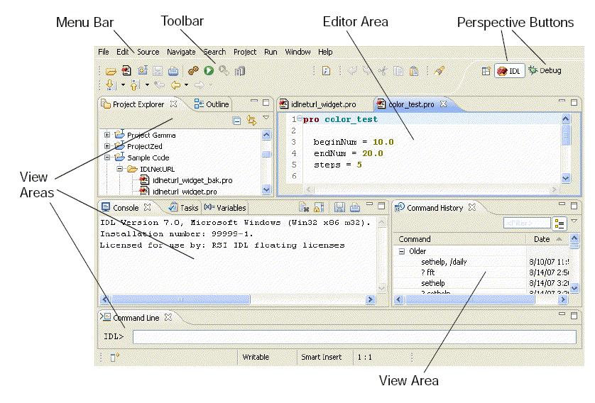
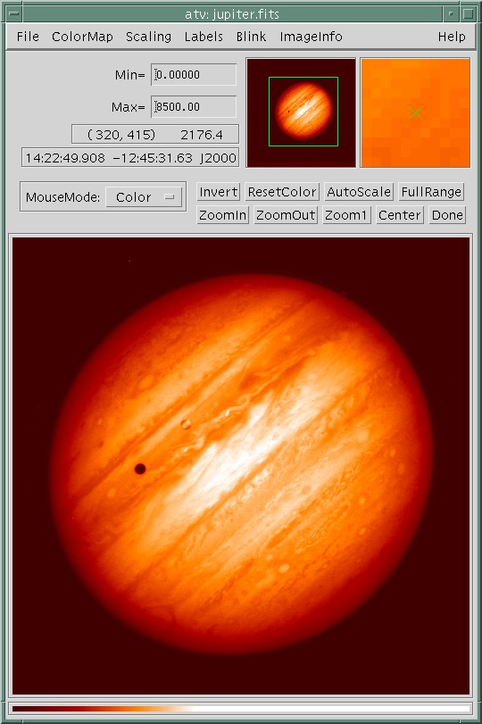